Automatic Spectral Segmentation

Radio-frequency scene analysis is much more complex than modulation recognition. A good first step is to blindly identify the frequency intervals for which significant non-noise energy exists.

In this post, I discuss a signal-processing algorithm that has almost nothing to do with cyclostationary signal processing (CSP). Almost. The topic is automatic spectral segmentation, which I also call band-of-interest (BOI) detection. When attempting to perform automatic radio-frequency scene analysis (RFSA), we may be confronted with a data block that contains multiple signals in a number of distinct frequency subbands. Moreover, these signals may be turning on and off within the data block. To apply our cyclostationary signal processing tools effectively, we would like to isolate these signals in time and frequency to the greatest extent possible using linear time-invariant filtering (for separating in the frequency dimension) and time-gating (for separating in the time dimension). Then the isolated signal components can be processed serially using CSP.

It is very important to remember that even perfect spectral and temporal segmentation will not solve the cochannel-signal problem. It is perfectly possible that an isolated subband will contain more than one cochannel signal.

The basics of my BOI-detection approach are published in a 2007 conference paper (My Papers [32]). I’ll describe this basic approach, illustrate it with examples relevant to RFSA, and also provide a few extensions of interest, including one that relates to cyclostationary signal processing.

The Problem

The efficacy of our cyclostationary signal processing (CSP) algorithms for any particular data record depends on several factors, including the noise power, interference power, processing block length, spectral resolution, and signal type. In general, it is better to apply CSP algorithms to a signal that has been filtered so that adjacent-channel signals and out-of-band noise are minimized. This just means that we want to minimize the “total SINR” of the data prior to CSP processing. By “total SINR” I simply mean the ratio of the signal power to the power of everything else in the data record, whether it has frequency content in the signal’s band or not.

This aim isn’t so hard to achieve when the input data consists of a single signal in white Gaussian noise (WGN). Then we need only apply a linear time-invariant filter to the data, where the center frequency and bandwidth of the filter match the center frequency and bandwidth of the signal. For example, consider a QPSK signal in noise. The PSD looks like this:

psd_qpsk — Figure 1. Power spectrum estimate for a noisy QPSK signal.

If we apply a simple Fourier-based linear time-invariant filter to that QPSK data, where the center frequency is zero and the width is $0.4$ Hz, we remove almost all of the out-of-band noise and retain the signal:

psd_qpsk_bpf — Figure 2. Power spectrum estimate for a filtered version of the noisy QPSK signal shown in Figure 1. Almost all of the noise that is out of the signal’s band of frequencies is eliminated by the filtering.

Removing the out-of-band noise won’t help much with estimating the spectral correlation function for the QPSK signal itself, because that will depend on the spectral components of the data that do in fact lie in the signal band. On the other hand, the SCF for frequencies $f$ that lie well outside the signal’s band is ideally zero, and will be easier to estimate when the out-of-band noise is removed.

But what about the temporal parameters like the cyclic autocorrelation and the cyclic cumulants? Well, they will be more sensitive to the presence of the out-of-band noise, because each point estimate takes into account all values of the input data block, so it is important to remove as much of it as possible prior to applying the estimator for the time-domain parameter of interest.

So we have reasons for wanting to apply simple signal processing methods to simple RF scenes like the QPSK signal above: increasing the total SNR improves estimator performance for fixed estimator parameters such as block length, spectral resolution etc. And increasing the total SNR means effectively locating the signal in the frequency domain and then applying a bandpass filter to that location.

The problems for our estimators get worse, however, when the scenarios aren’t simple.

Densely Populated RF Bands

In RF scene analysis, the goal of the signal processing algorithm is to blindly detect, classify, and characterize all signals present in the scene. No matter what the scene contains. Here is a sequence of PSDs for scenes of interest, where the scene complexity–measured by things like the number of signals present, the SINRs, and the noise-floor deviation from ideal–is increasing:

psd_fhdsss_data — Figure 3. Typical power spectrum estimate for a simulated hybrid FH/DSSS signal. On each visited carrier frequency (on each ‘hop’), the signal is DSSS.

psd_scene_5 — Figure 4. Power spectrum estimate for an RF scene containing multiple BPSK, QPSK, and MSK signals with decreasing symbol rate as the carrier is varied from left to right.

psd_fh_with_interf — Figure 5. Typical power spectrum estimate for an RF scene containing multiple frequency-hopped signals and intermittent wideband PSK interferers.

psd_acn — Figure 6. Power spectrum estimate for a complex multi-signal scene featuring single-signal and two-signal subbands and a wide variety of QAM/PSK/SQPSK signal types.

psd_pcs_882_50MHz — Figure 7. Typical power spectrum estimate for a captured RF scene in the PCS band near 880 MHz. The signal types are CDMA, LTE, WCDMA, and GSM.

psd_fm — Figure 8. Typical power spectrum estimate for a captured RF scene corresponding to the FM broadcast band in the United States. All signals in the scene are FM.

psd_testFile — Figure 9. Power spectrum estimate for a captured RF scene in the HF region of the spectrum.

By the time we get to the final few examples, we see collection-system filter roll-offs on the edges of the band, non-flat noise floors, high dynamic ranges in signal power and signal bandwidth, and closely spaced signals in frequency.

Distortion of Estimated Cumulants Due to Time-Gating

There is another reason to isolate a signal in the time and frequency domains prior to processing with CSP: distortion of sets of cyclic cumulants caused by partial signal temporal occupancy within a processed data block. (Awkwardly put, I know.)

Suppose we have a signal that exists only during a subset of the time instants corresponding to some sampled-data record. Let the subset occupy a fixed fraction $F$ of the data record, which itself spans the continuous-time interval $[-T/2, T/2]$ ,

$\displaystyle x(t) = s(t) + w(t), \ \ t \in [-T/2, T/2] \hfill (1)$

$\displaystyle s(t) = 0, t \not\in [e_1(T), e_2(T)], \hfill (2)$

$\displaystyle F = (e_2(T) - e_1(T))/T \hfill (3)$

Here $0 < F \leq 1$ and $w(t)$ is stationary white Gaussian noise. We use $F$ because it allows us to fix the fraction of time that the signal is on, relative to the interval $[-T/2, T/2]$ , so we can talk sensibly about the values of estimators as $T \rightarrow \infty$ . For example, if $e_1(T) = -T/2$ and $e_2(T) = T/2$ , then $F=1$ and we have our usual case where the signal persists over the entire observation (integration) interval. On the other hand, if $e_1(T) = -T/4$ and $e_2(T) = T/4$ , then $F = 1/2$ and the signal persists only over half of the observation interval.

Now we know that the temporal cumulant function is a particular sum of products of lower-order temporal moment functions,

$\displaystyle C_x(t, \boldmath{\tau}; n, m) = \sum_{P_n} (-1)^{p-1}(p-1)! \prod_{j=1}^n R_x(t, \boldmath{\tau}_j; n_j, m_m). \hfill (4)$

(See the post on cyclic cumulants for more information on this notation.)

Now the cumulant for $x(t)$ is the sum of the cumulant for $s(t)$ and $w(t)$ , and the latter is zero for $n \ge 3$ , so we focus on the cumulant for $s(t)$ . We’ll need the various lower-order cyclic moments (Fourier components of the time-varying moment $R_x(t,\boldmath{\tau}_j; n_j, m_j)$ ),

$\displaystyle R_{x_T}^{\alpha_n} (\boldmath{\tau}; n,m) = \frac{1}{T} \int_{-T/2}^{T/2} \prod_{j=1}^n s^{(*)_j} (t + \tau_j) e^{-i2\pi \alpha_n t} \, dt \hfill (5)$

Or, using $e_i(T)$ and $F$ ,

$\displaystyle R_{x_T}^{\alpha_n} (\boldmath{\tau}; n,m) = F \frac{1}{FT} \int_{e_1(T)}^{e_2(T)} \prod_{j=1}^n s^{(*)_j} (t+\tau_j) e^{-i2\pi \alpha_n t} \, dt \hfill (6)$

In the limit as $T\rightarrow \infty$ , we have

$\displaystyle R_{x}^{\alpha_n} (\boldmath{\tau}; n,m) = F R_s^{\alpha_n}(\boldmath{\tau}; n,m) \hfill (7)$

So the signal that persists only over a fraction of the observation interval is a scaled version of the signal that persists over the entire interval, and the scaling factor is quite reasonably $F = (e_2(T) - e_1(T))/T$ .

This implies that the temporal moment function is also scaled by $F$ ,

$\displaystyle R_x(t, \boldsymbol{\tau}; n,m) = F R_s(t, \tau; n,m) + R_w(t, \tau; n,m) \hfill (8)$

Keeping in mind that for higher orders the cumulant for $x(t)$ is that for $s(t)$ , we have

$\displaystyle C_x(t, \boldsymbol{\tau}; n,m) = \sum_{P_n} (-1)^{p-1}(p-1)! F^p \prod_{j=1}^p R_s(t, \boldsymbol{\tau}_j; n_j, m_j). \hfill (9)$

Unlike the temporal moment, the temporal cumulant is not simply a scaled version of that fully persistent signal–it is warped or distorted by the inclusion of $F^p$ , which is dependent on the partition size $p$ unless $F=1$ (the case in which the signal is persistent over the whole block).

So, processing involving linear combinations of multiple orders of moments is insensitive to $F < 1$ , but processing involving cumulants is not, because that involves different products of moments. Since my modulation-recognition algorithm is cumulant-based (see here, but more coming in a future post as well), this is an actual problem for me.

All of this implies that we need to include an interval-of-interest (IOI) estimator as well as a band-of-interest estimator in our spectral-segmentation algorithm. That way our calculations will always involve $F \approx 1$ once we estimate the IOI and time-gate the signal component accordingly.

Potential Solutions

A few others have created automatic spectral segmentation algorithms, or the equivalent, such as automatic noise-floor estimators that work for dense (crowded) RF scenes. One is The Literature [R96], which applies morphological image-processing operators (like erosion and dilation) to spectral data. Others, like The Literature [R97] advocate sophisticated high-resolution/high-accuracy spectrum estimators such as the multi-tapering method of The Literature [R98]. I think we do not need high spectrum-estimate accuracy here; the goal is to estimate the frequency intervals for which non-noise energy exists, not to obtain a super accurate spectrum estimate for all frequencies in the analysis band. So I’m of the opinion that high-performance spectrum estimators are out of place in the general band-of-interest estimation problem.

My Solution: Multiresolution Adaptive Spectrum Estimation

I outline the solution in My Papers [32]. The idea is to recursively apply a low-cost simple non-parametric power spectrum estimator to the input data record, which is assumed to contain $N$ complex samples and correspond to the complex envelope of some RF data (like the various spectra above).

Why “recursively?” In some cases, a wideband RF scene may contain several signals that are closely spaced in frequency. To see that there is a small gap between them requires that the spectral resolution of the spectrum estimator lies in a particular range. On the other hand, the scene may also (or only) contain a wideband signal with significant spectral variation across its bandwidth. In this latter case, there is only one band of interest, but the variability of a high-resolution spectrum estimate can make it appear that it is composed of multiple closely spaced bands of interest.

In other words, the required spectral resolution depends on the number and spacing of the signals in the scene, and we don’t want to make many assumptions about that.

What we do instead is to start out by applying a coarse spectral resolution to the data record, find the minima to estimate the noise floor, and declare everything else as bands of interest. Then, we apply the same algorithm to each of the detected BOIs, after filtering, frequency shifting, and decimating each one. This process will reveal which of the coarse lumps from the first spectrum estimate are really composed of multiple closely spaced BOIs and which are not.

I’ve found that this is a tricky idea to get across, so before we outline the mathematics of the algorithm, I want to further describe the multi-resolution idea with some pictures.

Consider the following multi-signal RF scene:

basic_psd_for_data — Figure 10. Power spectrum estimate for a band-of-interest performance evaluation input containing 21 signals with various bandwidths and a variety of band separations: Some are comfortably separated, some are nearly touching.

This scene contains $21$ individual signals, none of which overlap in frequency. This first PSD estimate for our $21$ -signal scene used the frequency-smoothing method and a smoothing-window width (spectral resolution) of $5000$ Hz ( $0.01$ Hz in normalized frequency). With this resolution, our eyes can count $11$ bands of interest, and we suspect the ones near $\pm 200$ kHz may contain several more. But the resolution is too coarse to reveal them in this picture.

More generally, let’s look at a sequence of PSD estimates for this scenario:

res_psds — Figure 11. Band-of-interest estimates for a non-interative version of the basic segmentation algorithm. The algorithm produces correct estimates only when the fixed spectral resolution of the estimator is well-matched to the more narrowband scene components.

In this sequence of PSD estimates, the spectral resolution is decreasing from top to bottom (the smoothing-window width in the FSM is increasing). The bands of interest are detected using only a single PSD estimate–no recursive processing is allowed. This shows that basic spectral segmentation algorithms fail when the PSD spectral resolution is not well-matched to the spectral variation exhibited by the underlying signals in the data.

The idea behind the automatic multi-resolution spectral segmentation algorithm is recursively applying a standard non-parametric PSD estimator (like the FSM), which I also call telescoping spectral estimation. For this $21$ -signal example, telescoping spectral segmentation is illustrated by the following diagram:

Figure 12. Illustration of the effect of iterating in the multi-resolution iterative band-of-interest estimator. The iterations cause a telescoping effect where a detected band of interest is examined with another application of the basic fixed-resolution algorithm to determine whether or not it contains multiple subbands of interest. This telescoping action continues until it is clear that a band consists of only a single subband.

When used on our $21$ -signal example, we obtain the following sequence of results:

res_multi_psds — Figure 13. Application of the multi-resolution iterative band-of-interest algorithm to the test input of Figure 11. Unlike the results for the fixed-resolution algorithm variant, the multi-resolution algorithm is insensitive to the particular spectral resolution used in the fixed-resolution algorithm at each iteration.

The indicated spectral resolution applies to the initial application of the non-parametric PSD estimator. Subsequent applications, as the telescoping action proceeds, use an effective resolution that has the same relation to the local sampling rate that the initial resolution has to the original sampling rate of $500$ kHz.

Here we see that the ability to correctly detect the $21$ bands of interest and to estimate the noise floor is only weakly dependent on the choice of spectral resolution.

Algorithm

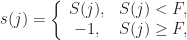
We first provide a fixed-resolution algorithm that finds bands of interest by defining them as arbitrary-shaped bumps that rise up from the noise floor. The multi-resolution version will follow.

In this algorithm statement, the $j$ th BOI has endpoints given by $[B_l(j-1), B_r(j-1)]$ .

Obtain data samples $x(i)$ , $i=0, \ldots, T-1$ .
Specify resolution ${\Delta \! f}_0$ (normalized frequency units).
Let $W = \lfloor T {\Delta \! f}_0 \rfloor$ . This is the width of the smoothing window in frequency bins.
Compute spectrum estimate with resolution product $T {\Delta \! f}_0$ , denote by $S(j)$ , $j = 0, \ldots, T-1$ .
$S_{min}$ is the minimum of $S(j)$ for $j \in [W/2, T-W/2)$ .
Denote by $F$ the noise-floor threshold $\eta S_{min}$ .
For each $j \in [W/2, T-W/2)$ : $s(j) = \left\{ \begin{array}{cc} S(j), & S(j) < F, \\ -1, & S(j) \ge F, \end{array} \right.$
Set $e = 0$ .
For each $j \in [W/2, T-W/2)$ , if $s(j) < 0$ and $s(j-1) \ge 0$ , set $B_l(e) = j$ . If $s(j) \ge 0$ and $s(j-1) < 0$ , set $B_r(e) = j$ and increment $e$ by $1$ .
If $s(W/2) = -1$ , then $B_l(0) = 0$ . (Handles BOI at left edge of PSD.)
If $s(T-W/2-1) = -1$ , then $B_r(e) = T-1$ . (Handles BOI at right edge of PSD.)
Estimate noise floor by computing the average value of PSD for all frequency points not assigned to a BOI interval.
Estimate power for BOI $k$ by summing PSD values for all frequency points assigned to BOI $k$ .
Remove weak BOIs, resulting in $N_b \le e$ BOIs.
BOI intervals are $[B_l(k), B_r(k)]$ , $k = 0, \ldots, N_b-1$ .
Stop.

We build on this fixed-resolution algorithm to create the recursive multi-resolution algorithm in the following way:

Obtain data samples $x(i)$ , $i=0, \ldots, T-1$ .
Specify nominal resolution ${\Delta \! f}_0$ .
Set $t = 0$ , $B(t, 1) = [-0.5, 0.5]$ , and $n_t = n_0 = 1$ .
Set $L(t, 1) = 0$ .
Set $j = 1$ .
Set $m = 0$ .
If $L(t, j) = 1$ , set $M=0$ and Goto Step 13.
Extract the BOI data from $x(i)$ that corresponds to $B(t,j)$ . Bandpass filter, downconvert, and decimate this data so that its fractional bandwidth is maximized and it is centered at zero frequency. The resulting data is $y(i)$ .
Estimate the PSD for $y(i)$ .
Use the fixed-resolution BOI detection algorithm with ${\Delta \! f}_0$ to find BOIs in $y(i)$ . Let the number of detected BOIs be $M$ .
Assign detected-BOI values to $B(t+1, k+m)$ , $k = 1, \ldots, M$ .
If $M = 1$ and $B(t, j) \approx B(t+1, m+1)$ , set $L(t+1, m+1) = 1$ , indicating the BOI is completed, else set $L(t+1, k+m) = 0$ for $k = 1, \ldots, M$ .
$m \rightarrow m + M$ .
$j \rightarrow j + 1$ .
If $j \leq n_t$ , then Goto Step 7.
$t \rightarrow t + 1$ .
Set $n_t = m$ .
If $L(t, k) = 0$ for any $k = 1, \ldots, n_t$ , Goto Step 6 else Stop.

When we apply this algorithm to the $21$ -BOI data file in a Monte Carlo simulation, we obtain the following performance graphs:

sam_harmonic_bois — Figure 14. Band-of-interest detection performance for the 21-BOI test input shown in Figure 11. Ideal performance consists of a mean of 21 detected BOIs and zero standard deviation.

sam_harmonic_N0 — Figure 15. Noise-floor estimate performance for the 21-BOI test input shown in Figure 10.

Here the total signal power is about $15$ dB, and the total power of the noise varies from $-10$ dB to $10$ dB.

Examples

Let’s apply the algorithm to the RF scenes I showed in the first several figures of the post. In all cases, the number of processed samples is $262144$ (regardless of the sampling rate) and the spectral resolution at each stage of recursion is $0.002$ times the effective sampling frequency at that stage.

sam_psd_qpsk — Figure 16. Application of the automatic spectral segmentation algorithm to the noisy QPSK signal shown in Figure 1.

sam_psd_fhdsss_data — Figure 17. Application of the automatic spectral segmentation algorithm to the hybrid FH/DSSS signal shown in Figure 3.

sam_psd_scene_5 — Figure 18. Application of the automatic spectral segmentation algorithm to the simulated-PSK scene shown in Figure 4.

sam_psd_fh_with_interf — Figure 19. Application of the automatic spectral segmentation algorithm to the simulated FH-plus-interferers scene shown in Figure 5.

sam_psd_acn — Figure 20. Application of the automatic spectral segmentation algorithm to the simulated congested cochannel scene shown in Figure 6.

sam_psd_pcs_882_50MHz — Figure 21. Application of the automatic spectral segmentation algorithm to the captured PCS scene shown in Figure 7.

sam_psd_fm — Figure 22. Application of the automatic spectral segmentation algorithm to the captured broadcast FM scene shown in Figure 8.

sam_psd_testFile — Figure 23. Application of the automatic spectral segmentation algorithm to the captured HF scene shown in Figure 9.

Extensions

Colored Noise

Several of the RF scenes above possess noise floors that are not flat throughout the analysis bandwidth. In particular, they have noise floors that decrease rather rapidly at the edges of the band. This is typically due to the action of a receiving system, which applies filtering prior to sampling. The applied filter bandwidth is smaller than the complex sampling rate, so that the band edges end up containing little energy. The noise is therefore not white (relative to the sampling rate), and so it is typically called colored. There are other deviations from white noise as well, such as tilted noise floors or those that contain ripples of various sorts. The most common is the filter-roll-off band-edge coloration, and the band-of-interest detector can handle that at the expense of increased computational cost.

The idea is to apply the basic algorithm to the data but restrict it to operate on a subband such as $[(-f_s/2+\Delta), (f_s/2-\Delta)]$ . Keep a count of the number of bands that are detected for each of several values of $\Delta$ . Retain only those bands that correspond to the maximum. When $\Delta = 0$ , the stated algorithm above will return a single band of interest, which is nearly the entire analysis band, because it will identify the noise floor as the value of the spectrum estimate very near $\pm f_s/2$ . In other words, the entire spectrum looks like one big band of interest having a very small noise floor. On the other hand, when $\Delta$ is such that only the flat part of the noise floor is considered, it will operate effectively and return all the true bands of interest that actually exist in the flat part, which is greater than or equal to one.

Interval-of-Interest Estimation

To perform the localization of signal components in the time domain, which I have called interval-of-interest estimation, I simply apply the algorithm developed for the band-of-interest estimation to the time-domain data itself. This is done for each detected band of interest separately. Interval-of-interest estimation is just the time-frequency dual algorithm to band-of-interest estimation.

Multi-Resolution Spectral Correlation Estimation for Targeted-Signal BOI Detection

The algorithm as discussed so far employs only power spectrum estimation–no cyclostationarity! A CSP extension is to replace the spectrum estimates with spectral correlation estimates. In fact, the entire algorithm above can be viewed as exploiting non-conjugate spectral correlation at a cycle frequency of $\alpha = 0$ . Why not choose a different value for $\alpha$ ? Such as one that corresponds to a cycle frequency for a signal that is being searched for? Then all bands that do not possess the desired cyclostationarity are ignored and are not processed, potentially saving significant computation.

There are a few complications, but the algorithm works for non-zero $\alpha$ . Let’s apply it to each of the scenes above, tailoring the choice for $\alpha$ according to the signals that we know exist in the scenes.

First, the simple single-signal scene involving QPSK. It has a symbol rate of $1/5$ , so we use that as the cycle frequency:

sam_psd_qpsk_xray — Figure 25. Multi-resolution band-of-interest detection using the spectral correlation function as applied to the noisy QPSK signal in Figure 1. Here the employed cycle frequency is the symbol rate of the QPSK signal.

Next up is the hybrid FH/DSSS signal, which possesses many cycle frequencies, but a prominent one is $0.02$ . Using this cycle frequency results in the following detection:

sam_psd_fhdsss_data_xray — Figure 26. Multi-resolution band-of-interest detection using the spectral correlation function as applied to the noisy hybrid FH/DSSS signal in Figure 3. Here the employed cycle frequency is a cycle frequency for the DSSS signal that persists over each hop duration.

Notice here there is a single detected band of interest rather than the two distinct bands produced by the main algorithm.

Next is the scene with the narrowband PSK/QAM signals. The leftmost signal in this scene is BPSK, and the fourth, seventh, etc. signals are also BPSK. The second, fifth, eighth, etc. are QPSK, and the remainder are SQPSK. The bandwidth of the signals is monotonically decreasing as the signal index moves from left to right, so that every signal has a unique symbol rate, which means a unique cycle frequency. We choose the bit rate of the third BPSK signal, the seventh signal from the left, which is $0.011$ . The result is:

sam_psd_scene_5_xray — Figure 27. Multi-resolution band-of-interest detection using the spectral correlation function as applied to the multi-component PSK/MSK scene in Figure 4. Here the employed cycle frequency is the symbol rate of the third BPSK signal from the left, which is the seventh band of interest from the left.

Now we turn to the scene containing an FH signal with intermittent wideband interferers. We choose the symbol rate of one of the interferers (situated near $-0.1$ Hz), which is $1/20$ :

sam_psd_fh_with_interf_xray — Figure 28. Multi-resolution band-of-interest detection using the spectral correlation function as applied to the FH scene in Figure 5. Here the employed cycle frequency is the symbol rate of one of the PSK interferers.

Next is the scene with a large number of signals of mixed bandwidth. We choose the symbol rate for the two signals between $-0.1$ and $0$ , which is $1/50$ , and this rate is not a cycle frequency for any of the other signals:

sam_psd_acn_xray — Figure 29. Multi-resolution band-of-interest detection using the spectral correlation function as applied to the simulated multi-component cochannel-signal scene in Figure 6. Here the employed cycle frequency is the symbol rate of the two signals with bands of interest between -0.1 and 0.0 Hz.

Turning now to captured data, we consider the PCS scene and choose the chip rate for CDMA, which is 1.2288 MHz. This cycle frequency is exhibited by the CDMA signals at $863$ and $893$ MHz, as well as by the CDMA-EVDO signal at $882$ MHz:

sam_psd_pcs_882_50MHz_xray — Figure 30. Multi-resolution band-of-interest detection using the spectral correlation function as applied to the captured PCS scene in Figure 7. Here the employed cycle frequency is the chip rate of CDMA, 1.2288 MHz. The two CDMA signals are detected as well as components of the CDMA EVDO signal near 882 MHz.

When we switch the cycle frequency to the WCDMA chip rate of $3.84$ MHz, we obtain the following bands of interest:

sam_psd_pcs_882_50MHz_2_xray — Figure 31. Multi-resolution band-of-interest detection using the spectral correlation function as applied to the captured PCS scene in Figure 7. Here the employed cycle frequency is the chip rate of WCDMA, 3.84 MHz. The two WCDMA signals are detected.

which makes sense because the two signals near $875$ MHz are indeed WCDMA.

The broadcast FM signals can exhibit a cycle frequency of $19.2$ kHz due to their digital components:

sam_psd_fm_xray — Figure 32. Multi-resolution band-of-interest detection using the spectral correlation function as applied to the captured broadcast FM scene in Figure 8. Here the employed cycle frequency is 19.2 kHz, which is associated with the digital component of modern broadcast FM signals.

As usual, if you find any errors in the post, please let me know in the comments. Questions are welcome, as always. I’m also very interested in knowing about any papers in the literature that present solutions to this general spectral segmentation problem.

Author: Chad Spooner

I'm a signal processing researcher specializing in cyclostationary signal processing (CSP) for communication signals. I hope to use this blog to help others with their cyclo-projects and to learn more about how CSP is being used and extended worldwide. View all posts by Chad Spooner

24 thoughts on “Automatic Spectral Segmentation”

Mirko von Leipzig says:

June 1, 2017 at 1:32 am

This is something I’ve struggled with a great deal myself. Developing an algorithm for real-world wideband signals of arbitrary sample rate is a major pain.

Most approaches I tried worked well at specific resolutions, but fail miserably at others.

I’ll try your approach and see how it compares to one I’ve made myself (recursively finds the biggest carrier until some SNR threshold is failed).

It would be interesting to see if this could be used to detect transponders – I have signals with multiple transponders – a PITA to analyse.

Reply
1. Mirko von Leipzig says:
  
  June 1, 2017 at 1:35 am
  
  (Some of your LaTeX math is displaying as raw string)
  
  Reply
  1. Chad Spooner says:
    
    June 1, 2017 at 8:27 am
    
    Thanks! I found two in the second algorithm statement…
    
    Reply
2. Mirko von Leipzig says:
  
  June 1, 2017 at 4:55 am
  
  How do you avoid missing smaller carriers in the rough FFT at the start?
  
  So an isolated carrier who’s power contribution will get lost compared to the noise in the FFT bin.
  
  Or does that dictate the resolution of our FFTs.
  
  Reply
  1. Chad Spooner says:
    
    June 1, 2017 at 8:34 am
    
    I do miss weaker signals. At some point, the power of a weak signal is comparable to the variance (fluctuations) in the spectral estimates, and it is very hard to tell the difference. So the basic algorithm definitely favors stronger signals. And that gets me pretty far. Your comment reminds me of an extension to the algorithm that I didn’t talk about, but might in an update. That is “white-space detection”, where we apply the algorithm as stated, but at the end, the bands of interest are defined as the spaces in-between the detected bands. We can view these as possibly noise-only bands. How to really tell? One way is to then apply CSP (for example, the SSCA) to these putative white spaces to see if there are cyclostationary signals lurking there. Computationally expensive though.
    
    Reply
3. Chad Spooner says:
  
  June 1, 2017 at 8:29 am
  
  I agree it is a difficult problem when the generality we’re aiming for is so high. And the algorithmic approach I’ve sketched is quite useful for me, but is far from perfect. There are so many variations on RF scenes that it seems impossible to construct an algorithm that works flawlessly on all of them. In particular, since the algorithm works by processing multiple (data-adaptive) spectrum estimates, it is in the end energy detection, and weaker signals are missed.
  
  Reply
Mirko von Leipzig says:

June 2, 2017 at 2:57 am

Could you expand on the complications in the last section (matching for specific cyclic frequencies)?

I’m getting lots of artifacts on real data (with many signals), where there isn’t any carrier. Could be due to carrier spacing relating to the cyclic frequency [X(f+a/2) X*(f-a/2)] creating energy?

I’m using the FSM method.

It works well for my simulated data.

Reply
1. Chad Spooner says:
  
  June 6, 2017 at 11:21 am
  
  Could you expand on the complications in the last section (matching for specific cyclic frequencies)?
  
  The complications arise from my definition of a band of interest as an arbitrary shaped bump between two flat spots. The flat spots correspond to noise-only intervals in the analysis band, and we can usually count on this because the noise is approximately flat across the entire band. So we can “drill down” until we hit the bedrock of the noise floor.
  
  When using spectral correlation to find BOIs, for spectral regions that don’t exhibit the chosen cycle frequency, there is no “flat spot”, because the spectral correlation there is ideally zero. So it becomes harder to tell where the edges of a band of interest are.
  
  Another problem is band-of-interest width estimation. Using the PSD, it is possible to estimate the band-of-interest width as the occupied bandwidth. Subsequent extraction of the band will generally capture almost all the signal energy, so downstream processing works. But with the spectral correlation function, recall that the width of the function can be quite a bit smaller than the occupied bandwidth. For example, for digital QAM/PSK with square-root raised-cosine pulses having roll-off $r$ and symbol rate $f_{sym}$ , the occupied bandwidth is $(1 + r)f_{sym}$ , but the width of the symbol-rate spectral correlation feature is just $rf_{sym}$ .
  
  I’m getting lots of artifacts on real data (with many signals), where there isn’t any carrier. Could be due to carrier spacing relating to the cyclic frequency [X(f+a/2) X*(f-a/2)] creating energy?
  
  But what is the cycle frequency $a$ here, and how far apart are distinct signals? It is hard to reply without specifics. Are you using the coherence or the spectral correlation to try to detect BOIs? I also find artifacts are common if there are very narrowband signals present (like tones). These create havoc especially for the coherence function.
  
  Reply
  1. Mirko von Leipzig says:
    
    June 7, 2017 at 1:29 am
    
    I’ve found that I can determine all symbol rates of interest present in a wideband signal using FFT(|x|) given enough data. I was using these as alpha. The nice thing about this is that I know what bandwidths I’m looking for (i.e. symbol rate plus some roll off).
    
    Worst case scenario is for signals to have their 3dB bandwidths touching. Tones (i.e. satellite beacons) are causing havoc yes; but so are carriers of different bandwidths that just happen to be a/2 apart.
    
    I’m straight up just using X(f+a/2) X*(f-a/2). So I suppose that makes it the spectral correlation. Should I be using coherence?
    
    Reply
    1. Chad Spooner says:
      
      June 8, 2017 at 10:44 am
      
      I’m intrigued by the use of the absolute value… contains various nonlinearities in one shot.
      
      but so are carriers of different bandwidths that just happen to be a/2 apart.
      
      Ah. Suppose $a$ is a symbol rate for some signal in the data. If there are two signals with center frequencies separated by $a$ , then spectral correlation may be present due to some correlation between the two different signals. In other words, suppose the two signals are statistically independent (and therefore uncorrelated). Then if you pick frequencies $f$ in the region that is about halfway between the two carriers, and the cycle frequency $a$ , you should NOT see significant non-conjugate spectral correlation. However, if the two signals have some information in common, you very well might see spectral correlation. For example, if the two signals are transferring independent user data streams, but use the same periodically repeated training sequence (for, say, channel equalization) or some other in-common data, then you can see spectral correlation. So that would definitely confuse an automatic spectral segmentation algorithm using $a$ or a cycle detector.
      
      Coherence, as opposed to spectral correlation, won’t help in this case, because there really is spectral correlation there, so the coherence will reflect that too. In general, I tend to use coherence as a detection statistic for cycle-frequency detection (as opposed to the cycle detectors) because of the relative ease of threshold computation. (A post on that is forthcoming, but see the comments on the SSCA post.)
      
      Reply
Sorin Goldenberg says:

August 21, 2017 at 11:04 pm

I come back to this problem once in a while.
Two thoughts that I have (and I lack the knowledge to answer them).
Seems we humans would quite easily be able to separate between signals in spectrum. Is there a way to transform it to an AI / image processing problem?
Trying to determine BOIs – I wonder if there is any property of a signal such that two separate sub-bands can be identified as being part of one single signal?

Reply
1. Chad Spooner says:
  
  August 22, 2017 at 9:46 am
  
  Hey Sorin. Thanks for commenting. Yes, when I first started trying to construct an algorithm for automatic BOI estimation, I tried to formulate how I went about identifying BOIs when I stared at a PSD estimate. I came up with nothing profound: a BOI is a arbitrary-shaped bump between two flat spots. All of the subsequent work is trying to ensure that I can identify flat spots! Not as easy as it sounds once we look at real data sets from receivers with imperfections and spectral bands with strange goings-on, not to mention the dependence of the flatness on the parameters of the non-parametric PSD estimator.
  
  One of the papers I referenced in the post tries to apply some image-processing tools to the BOI estimation problem. Not in an AI context though.
  
  The second point you bring up, about trying to group two or more seemingly separate (in frequency) BOIs, is something I’ve tackled as well. The first time was in the context of textbook rectangular-pulse PSK/QAM and textbook MFSK. Each has significant sidelobes. Essentially I use symmetry to try to group bands together. Another context is a signal that is frequency hopping. You’d like to group (associate) all the individual BOIs that you might detect over time and frequency. I have ways of doing this that work well enough for simple FH models, but they are not foolproof, as they rely solely on spectrogram-like analysis (no CSP!).
  
  Finally, I suppose if you can find the BOIs, interrogate their contents using CSP, then you might be able to group disparate BOIs together based on their shared cycle frequencies.
  
  Reply
  1. Sorin Goldenberg says:
    
    August 22, 2017 at 12:04 pm
    
    What about signals with more complex spectrum – like CPM/CPFSK that don’t look as nice as sqrtrc QAM/PSK? Or non line of sight signals that have a deep notch in the spectrum. How would you be able to decide if this is one signal or more, based on the shape alone.
    
    Reply
    1. Chad Spooner says:
      
      August 26, 2017 at 9:09 am
      
      I think the spectrum-based approach will fail for a lot of these kinds of cases. You can always come up with a propagation channel and ideal spectrum shape that when combined yields a measurable spectrum that looks exactly like the spectrum of two adjacent-channel signals. So, I admit failure! The multi-resolution spectrum-estimation approach I’ve outlined (and use every day!) cannot, by itself, resolve all ambiguities. Sigh. I suppose, however, you might do better if you can use additional information, such as the patterns of cycle frequencies that you see by (1) processing each “signal” separately, and (2) processing them after forcing them to be joined together. But that is going to cost some CPU cycles.
      
      For signals with multi-modal spectra (like some CPM and traditional FSK signals), if the valleys between the peaks aren’t too shallow, we can still detect the correct full signal band with this kind of PSD-based approach. But once those valleys get small (near zero for a noiseless signal PSD), then my method will start to declare them as separate signals.
      
      In fact, when I apply it to a textbook rectangular-pulse PSK signal, I often get an output consisting of a separate BOI for each of the sidelobes. Thankfully, I do not often encounter such spectra in captured data.
      
      Reply
Marty Ryba says:

February 27, 2018 at 11:18 am

Hi Chad, I’m having a bit of trouble following your notation to try out this approach as compared to one I’m currently using. Do you have any example code (e.g., MATLAB)? Can this iterative algorithm work with a “baseline” PSD at a nominal high resolution and the compute the windowed spectra off that? I can have FPGA firmware accumulate up the PSD but it certainly appears that this type of algorithm requires software. An interesting low-cost addition is to “filter” the PSD with a non-linear denoising algorithm like Total Variance which can remove the fuzz but preserve the larger excursions.

Reply
1. Chad Spooner says:
  
  February 28, 2018 at 9:28 am
  
  Thanks for the comment Marty, and for visiting the CSP Blog.
  
  I don’t have automatic spectral segmentation code for you, and I’m truly sorry for the difficult notation. Do you think there is an error using the notation or an inconsistency? The telescoping action makes it hard to write the algorithm in a readable way.
  
  Can this iterative algorithm work with a “baseline” PSD at a nominal high resolution and the compute the windowed spectra off that?
  
  No, the algorithm requires access to the data itself to perform the successive PSD estimates as it telescopes.
  
  I can have FPGA firmware accumulate up the PSD but it certainly appears that this type of algorithm requires software.
  
  I’m no hardware or FPGA expert, but it does seem to me this is a logic-heavy and iterative algorithm with an input-data-dependent number of iterations. I’ve certainly not convinced anybody to try to implement it in an FPGA.
  
  Maybe your best option is to just try to take the core idea, of telescoping or multiresolution/iterative spectrum estimation and try to make your own version of the algorithm?
  
  Can you provide a link to what you mean by the Total Variance Denoising algorithm?
  
  Reply
Marty Ryba says:

February 28, 2018 at 9:52 am

Thanks for the clarification Chad, I’m having someone look to build something from your 2007 paper, or use it for inspiration for an approach that starts with an accumulated PSD. An FPGA is pretty efficient in running multiple FFTs and then accumulating the results for a fixed transform size. If I accumulate a couple hundred FFT frames the PSD noise drops to below 0.5 dB so I have a nice clean spectrum to start with.

A good place to look over some denoising algorithms is the work by Dr. Ivan Selesnick at NYU. http://eeweb.poly.edu/iselesni/research/index.html

Reply
Rob says:

May 4, 2021 at 3:13 am

Dear Chad,

Could you please explain me why, in your first algorithm, step 11, B_r(e) = T-1 and not B_r(e) = T-W/2-1 ?
Also, did you have any insight concerning the fft(|x|) method that has been proposed in the comments? I’ve tested on a couple of signals I had around, and it managed to have a nice peak spot on the symbol rate (sheer luck ??) — that would be a game changer, as it would be much more computationally efficient that doing CSP…
Thanks and have a nice day ! 🙂
Rob

Reply
1. Chad Spooner says:
  
  May 4, 2021 at 2:29 pm
  
  Could you please explain me why, in your first algorithm, step 11, B_r(e) = T-1 and not B_r(e) = T-W/2-1 ?
  
  I restrict the computation of $s(\cdot)$ to [ $W/2$ , $T-W/2$ ] because I’m using the FSM, and I want to avoid testing the edges of the PSD for high values relative to the noise floor. This is because the edges of the PSD are distorted by the rectangular smoothing window in the FSM, so they can’t really reflect the noise floor value without some additional effort, and also there might be a BOI there. Which you probably already understood since you didn’t ask about that! But that means the rightmost frequency I check for BOI-hood has index $T-W/2$ . If that frequency bin has PSD that exceeds the threshold, then I simply assume that the BOI extends past $T-W/2$ and may go all the way to $T-1$ , the final frequency index. Similarly, in Step 10 if the first checked frequency has PSD that exceeds the threshold, then I simply assume the BOI extends to the left to the first frequency index of $0$ .
  
  did you have any insight concerning the fft(|x|) method that has been proposed in the comments?
  
  Looking at the Fourier transform of $x^(t)$ or $x^4(t)$ or $|x(t)|$ can certainly provide a peak at one or more cycle frequencies, and I consider this “doing CSP.” However, it devolves to peak-picking, so I find the spectral coherence more useful over a very wide range of scenarios, SNRs, and SINRs. The correntropy crowd wants to do a similar thing with $exp(|x(t|)$ , trying to get at all the second- and higher-order cycle frequencies in one shot, and providing tolerance to impulsive noise. See my comments on that approach here and here.
  
  Reply
  1. Rob says:
    
    May 4, 2021 at 9:51 pm
    
    Super-detailed and super-helpful explanations — as usual!
    Thanks a lot!! 🙂
    Rob
    
    Reply
  2. Laura says:
    
    July 11, 2023 at 3:04 pm
    
    Hi Chad,
    
    Based on this comment, it seems like you perform a linear convolution when smoothing in your FSM algorithm. Would it be a good idea to perform a circular convolution instead? I can see how problems would arise if out-of-band signals partially impinging on the receiver bandwidth may cause artifacts at the edges of the PSD. However, wouldn’t a circular convolution lead to a (maybe imperceptibly) better estimate of a cycle frequency?
    
    Thanks
    Laura
    
    Reply
    1. Chad Spooner says:
      
      July 12, 2023 at 4:29 pm
      
      it seems like you perform a linear convolution when smoothing in your FSM algorithm
      
      Yes.
      
      I can see how problems would arise if out-of-band signals partially impinging on the receiver bandwidth may cause artifacts at the edges of the PSD
      
      Yes, and remember that the algorithm is iterative–it telescopes onto the detected BOIs at level n, trying to resolve them more finely at level n+1. So at each level, I want to avoid the edges of the corresponding FSM-produced PSD.
      
      wouldn’t a circular convolution lead to a (maybe imperceptibly) better estimate of a cycle frequency?
      
      All I’m trying to do here is estimate intervals (ordered pairs $\displaystyle [f_{i, min}, f_{i, max}]$ ). Can you elaborate on how you think cycle frequencies, which are estimated downstream after extracting complex envelopes defined by the estimated frequency intervals, would be better estimated with a different convolution in the segmenter? Maybe I’m missing something helpful!
      
      Reply
Maggiee says:

November 21, 2023 at 1:23 am

Hi Chad!

As per your suggestion, I was browsing through your paper “Multi-Resolution White-Space Detection for Cognitive Radio” and this blog. And I have some simple questions regarding BOI detection Fixed-Resolution Algorithm.

How are the $\eta S_{min}$ mentioned therein determined? For example, when we get a signal we can calculate its PSD and by observation we can find the noise-floor or the bandwidth, but if we have to process 100 samples of this kind signal at a time, how do we determine the $\eta S_{min}$ value for each signal at once? When we can’t observe them one by one?

Thank you for your instruction

Reply
1. Chad Spooner says:
  
  November 21, 2023 at 5:12 pm
  
  The value of $S_{min}$ is just the minimum value of the PSD estimate, excluding the edges if using the FSM.
  
  The value of $\eta$ is a design parameter and relates to the expected variance of the PSD estimate, which depends on the algorithm parameters used (e.g., the smoothing window width in the FSM) and the total number of processed samples. See Figure 15 for some noise-floor mean and standard deviation results using the FSM. Also, you might want to look at the post on the resolution product.
  
  if we have to process 100 samples of this kind signal at a time, how do we determine the value for each signal at once? When we can’t observe them one by one?
  
  I recommend processing RF scenes using more than 100 samples, no matter what the bandwidth is. The variability of the noise-floor estimate is inversely proportional to the spectral resolution of the PSD estimate as well as the total number of processed samples (see the resolution product post). Using a small number of samples will result in a very high variability, and so random fluctuations in the noise floor will be mistaken for bands of interest (signals).
  
  I don’t grasp the meaning of “we can’t observe them one by one.” Can you elaborate?
  
  In my default band-of-interest detection algorithm, I use $\eta = 1.25$ . Remember that the threshold $\eta S_{min}$ is applied to PSD values to find the bands of interest, and $S_{min}$ is not an estimate of $N_0$ , it is the minimum PSD estimate. So to find values of the PSD that are likely not just noise floor, you have to exceed $S_{min}$ by a couple standard deviations or so.
  
  Reply