
In this post, we look at the ability of various CSP estimators to distinguish cycle frequencies, temporal changes in cyclostationarity, and spectral features. These abilities are quantified by the resolution properties of CSP estimators.
Resolution Parameters in CSP: Preview
Consider performing some CSP estimation task, such as using the frequency-smoothing method, time-smoothing method, or strip spectral correlation analyzer method of estimating the spectral correlation function. The estimate employs 
Then the temporal resolution 


What do we usually mean by spectral resolution as the term is used in conventional spectrum analysis? It sums up the ability of the estimator to display distinct responses to data components that have distinct spectra. That idea is somewhat abstract, so spectral resolution is often described more concretely as the ability of the estimator to reveal the presence of two closely spaced spectral components from, typically, two equal-strength sine waves at the estimator input.
Spectral Resolution in the Periodogram
The estimators I’m interested in are variants of the two basic non-parametric spectrum estimators that apply either time smoothing (temporal averaging) or frequency smoothing (spectral averaging) to the periodogram. The former is called the time-smoothing method and the latter the frequency-smoothing method of spectrum estimation, although there are the alternate names involving Proper Nouns that some people prefer: the Bartlett and Daniell methods.
Both methods take as the starting point a periodogram. In the case of the time-smoothing method, multiple periodograms are computed and averaged over time, so that the spectral resolution of the result must be the spectral resolution of the involved periodograms. In the case of the frequency-smoothing method, a single periodogram is convolved with a pulse-like smoothing kernel, so that the spectral resolution cannot be smaller than the native spectral resolution of the involved periodogram, and is equal to the width of the pulse-like kernel. So we must start with understanding the spectral resolution properties of the periodogram.
Let’s review the periodogram. First, we define the sliding (over time) finite-time Fourier transform as

The periodogram is the scaled squared magnitude of this quantity:

What is the frequency resolution of this estimator? Since it integrates over a total of
Consider a noiseless input 


What is the periodogram for this input? Let’s first calculate the sliding Fourier transform 


If 


![\displaystyle = \frac{A_0 e^{i\phi_0}}{-i2\pi (f-f_0)} \left[ e^{-i2\pi(f-f_0)(t+T/2)} - e^{-i2\pi(f-f_0)(t-T/2)} \right] \hfill (7)](https://s0.wp.com/latex.php?latex=%5Cdisplaystyle+%3D+%5Cfrac%7BA_0+e%5E%7Bi%5Cphi_0%7D%7D%7B-i2%5Cpi+%28f-f_0%29%7D+%5Cleft%5B+e%5E%7B-i2%5Cpi%28f-f_0%29%28t%2BT%2F2%29%7D+-+e%5E%7B-i2%5Cpi%28f-f_0%29%28t-T%2F2%29%7D+%5Cright%5D+%5Chfill+%287%29&bg=ffffff&fg=1a1a1a&s=0&c=20201002)
![\displaystyle = \frac{A_0 e^{i\phi_0}}{-i2\pi (f-f_0)} e^{-i 2 \pi (f-f_0)t} \left[ e^{-i2\pi(f-f_0)T/2} - e^{i2\pi(f-f_0)T/2} \right] \hfill (8)](https://s0.wp.com/latex.php?latex=%5Cdisplaystyle+%3D+%5Cfrac%7BA_0+e%5E%7Bi%5Cphi_0%7D%7D%7B-i2%5Cpi+%28f-f_0%29%7D+e%5E%7B-i+2+%5Cpi+%28f-f_0%29t%7D+%5Cleft%5B+e%5E%7B-i2%5Cpi%28f-f_0%29T%2F2%7D+-+e%5E%7Bi2%5Cpi%28f-f_0%29T%2F2%7D+%5Cright%5D+%5Chfill+%288%29&bg=ffffff&fg=1a1a1a&s=0&c=20201002)
Now, we can use Euler’s formula to simplify the term in the square brackets,

Application of (9) in (8) leads to
![\displaystyle X_T(t,f) = \frac{A_0 e^{i\phi_0}}{-i2\pi (f-f_0)} e^{-i 2 \pi (f-f_0)t} \sin(2\pi[f-f_0]T/2) \hfill (10)](https://s0.wp.com/latex.php?latex=%5Cdisplaystyle+X_T%28t%2Cf%29+%3D+%5Cfrac%7BA_0+e%5E%7Bi%5Cphi_0%7D%7D%7B-i2%5Cpi+%28f-f_0%29%7D+e%5E%7B-i+2+%5Cpi+%28f-f_0%29t%7D+%5Csin%282%5Cpi%5Bf-f_0%5DT%2F2%29+%5Chfill+%2810%29&bg=ffffff&fg=1a1a1a&s=0&c=20201002)
![\displaystyle = TA_0 e^{i\phi_0} e^{-i 2 \pi (f-f_0)t} \left[ \frac{\sin(\pi[f-f_0]T)}{\pi (f-f_0)T} \right] \hfill (11)](https://s0.wp.com/latex.php?latex=%5Cdisplaystyle+%3D+TA_0+e%5E%7Bi%5Cphi_0%7D+e%5E%7B-i+2+%5Cpi+%28f-f_0%29t%7D+%5Cleft%5B+%5Cfrac%7B%5Csin%28%5Cpi%5Bf-f_0%5DT%29%7D%7B%5Cpi+%28f-f_0%29T%7D+%5Cright%5D+%5Chfill+%2811%29&bg=ffffff&fg=1a1a1a&s=0&c=20201002)
We recognize the function in the square brackets as the sinc function, which is defined by

so that our time-varying Fourier transform is given by
![\displaystyle X_T(t,f) = TA_0e^{i \phi_0} e^{-i 2 \pi (f-f_0)t} {\rm \ sinc}([f-f_0]T) \hfill (13)](https://s0.wp.com/latex.php?latex=%5Cdisplaystyle+X_T%28t%2Cf%29+%3D+TA_0e%5E%7Bi+%5Cphi_0%7D+e%5E%7B-i+2+%5Cpi+%28f-f_0%29t%7D+%7B%5Crm+%5C+sinc%7D%28%5Bf-f_0%5DT%29+%5Chfill+%2813%29&bg=ffffff&fg=1a1a1a&s=0&c=20201002)
For 
![{\rm sinc}([f-f_0]T) = {\rm sinc}(0) = 1](https://s0.wp.com/latex.php?latex=%7B%5Crm+sinc%7D%28%5Bf-f_0%5DT%29+%3D+%7B%5Crm+sinc%7D%280%29+%3D+1&bg=ffffff&fg=1a1a1a&s=0&c=20201002)


The figure indicates that the transform peaks at the correct frequency, but that the transform is also non-zero for a great many other frequencies–frequencies that are not present in the tone itself. This frequency response arises due to the finite-time window of the transform, because we know that the Fourier transform (which is taken over all time) for the noiseless tone is an impulse function centered at 
Now, the periodogram is given by

so that the periodogram for our noiseless tone is simply
![\displaystyle I_T(t,f) = \frac{1}{T} A_0^2 T^2 {\rm \ sinc}^2([f-f_0]T) \hfill (15)](https://s0.wp.com/latex.php?latex=%5Cdisplaystyle+I_T%28t%2Cf%29+%3D+%5Cfrac%7B1%7D%7BT%7D+A_0%5E2+T%5E2+%7B%5Crm+%5C+sinc%7D%5E2%28%5Bf-f_0%5DT%29+%5Chfill+%2815%29&bg=ffffff&fg=1a1a1a&s=0&c=20201002)
![\displaystyle = A_0^2 T {\rm \ sinc}^2 ([f-f_0]T) \hfill (16)](https://s0.wp.com/latex.php?latex=%5Cdisplaystyle+%3D+A_0%5E2+T+%7B%5Crm+%5C+sinc%7D%5E2+%28%5Bf-f_0%5DT%29+%5Chfill+%2816%29&bg=ffffff&fg=1a1a1a&s=0&c=20201002)
This periodogram is plotted in the following figure:

 samples of a noiseless sine wave with frequency 0.05 and unit amplitude. The Fourier transform that is used to compute the periodogram uses 256 samples. Note that the periodogram is significant for many frequencies near to the sine-wave frequency of 0.05, but gets quite small for far-away frequencies.
We see that the width of the main lobe of this function is 
Now, let’s get back to talking about spectral resolution. What is the periodogram for the case of a signal consisting of two tones? The signal model is

The Fourier integral is linear, so we can immediately generalize our previous result for 
![\displaystyle X_T(t, f) = \sum_{j=0}^1 A_j T e^{i\phi_j} e^{-i2\pi (f-f_j)t} {\rm \ sinc}([f-f_j]T) \hfill (18)](https://s0.wp.com/latex.php?latex=%5Cdisplaystyle+X_T%28t%2C+f%29+%3D+%5Csum_%7Bj%3D0%7D%5E1+A_j+T+e%5E%7Bi%5Cphi_j%7D+e%5E%7B-i2%5Cpi+%28f-f_j%29t%7D+%7B%5Crm+%5C+sinc%7D%28%5Bf-f_j%5DT%29+%5Chfill+%2818%29&bg=ffffff&fg=1a1a1a&s=0&c=20201002)
and we can use this expression for 
![\displaystyle = T \sum_{j=0}^1 A_j^2 {\rm \ sinc}^2([f-f_j]T) + 2 \Re \left[ A_0A_1Te^{i(\phi_0 - \phi_1)} e^{-i2\pi(f_1 - f_0)t} {\rm\ sinc}([f-f_0]T) {\rm\ sinc}([f-f_1]T) \right] \hfill (19)](https://s0.wp.com/latex.php?latex=%5Cdisplaystyle+%3D+T+%5Csum_%7Bj%3D0%7D%5E1+A_j%5E2+%7B%5Crm+%5C+sinc%7D%5E2%28%5Bf-f_j%5DT%29+%2B+2+%5CRe+%5Cleft%5B+A_0A_1Te%5E%7Bi%28%5Cphi_0+-+%5Cphi_1%29%7D+e%5E%7B-i2%5Cpi%28f_1+-+f_0%29t%7D+%7B%5Crm%5C+sinc%7D%28%5Bf-f_0%5DT%29+%7B%5Crm%5C+sinc%7D%28%5Bf-f_1%5DT%29+%5Cright%5D+%5Chfill+%2819%29&bg=ffffff&fg=1a1a1a&s=0&c=20201002)
We see there is a sinc function centered at 
In the case of 
What about inbetween?
The squared-sinc terms represent the responses to each tone as if it were the only tone present, and do not depend on time 


![\displaystyle 2A_0 A_1 T {\rm \ sinc}([f-f_0]T) {\rm \ sinc} ([f-f_1]T). \hfill (20)](https://s0.wp.com/latex.php?latex=%5Cdisplaystyle+2A_0+A_1+T+%7B%5Crm+%5C+sinc%7D%28%5Bf-f_0%5DT%29+%7B%5Crm+%5C+sinc%7D+%28%5Bf-f_1%5DT%29.+%5Chfill+%2820%29&bg=ffffff&fg=1a1a1a&s=0&c=20201002)
The best case is when 

We can numerically evaluate these two extremes and plot the results to determine, approximately, the resolvability of the two tones as a function of their difference and the observation interval length 


First, the best-case version of the periodogram formula (19):

Here we see that two distinct peaks in the periodogram are visible for 

The worst-case version of formula (19) is computed and graphed in the following figure:

Here the two tones show two distinct peaks for 
Summing up, the resolution of the periodogram is about
Spectral Resolution in Non-Parametric Spectrum Estimators
Now that we know something about the spectral resolution of the periodogram, and since we know how the periodogram is related to important spectrum estimators, we can discuss the spectral resolution of these estimators.
For the frequency-smoothing method of PSD estimation, the periodogram is convolved with a smoothing function 
For the time-smoothing method of PSD estimation, multiple short-time periodograms are averaged over time. If 


Spectral Resolution in the Cyclic Periodogram
It is probably intuitive for my readers to see that the spectral resolution of the cyclic periodogram is about equal to the spectral resolution of the periodogram. In fact, the (non-conjugate) cyclic periodogram is identically equal to the periodogram for 
Spectral Resolution in Non-Parametric Spectral Correlation Estimators
Like the spectral estimators, the spectral correlation estimators will have spectral resolution that is determined by the averaging that is applied to the cyclic periodogram. For the frequency-smoothing method, it will be approximately the width of the smoothing kernel function, and for the time-smoothing method, it will be the reciprocal of the periodogram length
But let’s verify and illustrate these claims before leaving the topic of spectral resolution and moving to temporal and cycle-frequency resolution. Here it is harder to illustrate the situation using tone inputs (why?), so we look at a signal that has significant variation over frequency for both its spectrum and its spectral correlation function: the direct-sequence spread-spectrum BPSK signal. Let’s consider a DSSS BPSK signal with chip rate 


We start with estimates of the PSD, the chip-rate non-conjugate SCF, and the data-rate non-conjugate SCF using a very long version of the signal and a very small smoothing-kernel width in the FSM. This produces a set of reference (high-fidelity) estimates useful for later comparison with other estimates. Here are the reference estimates:

Note here that the three SCF estimates have several very narrow spectral features (nulls). Unlike the case of the periodogram, where we looked at the ability to distinguish two peaks in the spectrum, here we look at the ability to accurately estimate a narrow valley. Either way, we are trying to resolve something (distinguish something from something else).
First, let’s look at a sequence of FSM estimates, where we vary the width of the smoothing kernel

By studying these plots, you can see that the basic claim is verified: The spectral resolution is approximately equal to the width of the smoothing kernel. That is probably unsurprising and somewhat obvious to most readers, who are likely quite familiar with convolution and its smearing/smoothing effects. Let’s repeat this experiment, then, with the TSM, which employs no convolution at all:

Temporal Resolution in Non-Parametric CSP Estimators
The temporal resolution
Temporal resolution is a little hard to talk about in the context of our usual definitions of parameters such as the cyclic autocorrelation or spectral correlation function, because those definitions involve averaging over an infinite amount of time. If we consider finite-time estimates, and also consider a sequence of such estimates arising from processing a sequence of non-overlapping adjacent contiguous data blocks, then we can consider the ability of the sequence of estimates to resolve any changes in the parameter over time.
From this point of view, it seems clear that the temporal resolution
Cycle-Frequency Resolution in the Context of the Cyclic Autocorrelation Function
Now let’s turn to resolution in cycle frequency. In particular, let’s first look at the cyclic autocorrelation function. I’ll be focusing on the non-conjugate CAF, but all of what follows is applicable to the conjugate CAF too.
Recall that the non-conjugate CAF is defined as a Fourier coefficient in the Fourier series expansion of the time-variant autocorrelation function. It is also equal to the following limit

A natural and effective estimator is simply the finite-time version of this idealized average.
The lag product 

where

But this kind of representation must also be true for each cycle frequency 

with

and

So an estimate of the cyclic autocorrelation function for cycle frequency
![\displaystyle \hat{R}_x^\alpha(\tau) = \frac{1}{T} \int_{-T/2}^{T/2} \left[ R_x(t, \tau) + E(t, \tau) \right] e^{-i2\pi\alpha t} \, dt \hfill (27)](https://s0.wp.com/latex.php?latex=%5Cdisplaystyle+%5Chat%7BR%7D_x%5E%5Calpha%28%5Ctau%29+%3D+%5Cfrac%7B1%7D%7BT%7D+%5Cint_%7B-T%2F2%7D%5E%7BT%2F2%7D+%5Cleft%5B+R_x%28t%2C+%5Ctau%29+%2B+E%28t%2C+%5Ctau%29+%5Cright%5D+e%5E%7B-i2%5Cpi%5Calpha+t%7D+%5C%2C+dt+%5Chfill+%2827%29&bg=ffffff&fg=1a1a1a&s=0&c=20201002)
Neglecting 


If 

![\displaystyle = \left( \frac{1}{-i2\pi(\alpha-\beta)} \right) \left[ e^{-i2\pi(\alpha-\beta)T/2} - e^{i2\pi(\alpha-\beta)T/2} \right]](https://s0.wp.com/latex.php?latex=%5Cdisplaystyle+%3D+%5Cleft%28+%5Cfrac%7B1%7D%7B-i2%5Cpi%28%5Calpha-%5Cbeta%29%7D+%5Cright%29+%5Cleft%5B+e%5E%7B-i2%5Cpi%28%5Calpha-%5Cbeta%29T%2F2%7D+-+e%5E%7Bi2%5Cpi%28%5Calpha-%5Cbeta%29T%2F2%7D+%5Cright%5D+&bg=ffffff&fg=1a1a1a&s=0&c=20201002)
![\displaystyle = \frac{\sin(\pi[\alpha-\beta]T)}{\pi (\alpha-\beta)} = T{\rm sinc}([\alpha-\beta]T). \hfill (30)](https://s0.wp.com/latex.php?latex=%5Cdisplaystyle+%3D+%5Cfrac%7B%5Csin%28%5Cpi%5B%5Calpha-%5Cbeta%5DT%29%7D%7B%5Cpi+%28%5Calpha-%5Cbeta%29%7D+%3D+T%7B%5Crm+sinc%7D%28%5B%5Calpha-%5Cbeta%5DT%29.+%5Chfill+%2830%29&bg=ffffff&fg=1a1a1a&s=0&c=20201002)
Turning back to the CAF estimate, we now have
![\displaystyle \hat{R}_x^\alpha(\tau) \approx R_x^\alpha(\tau) + \sum_{\beta, \beta\neq\alpha} R_x^\beta(\tau) {\rm sinc}([\alpha-\beta]T) \hfill (31)](https://s0.wp.com/latex.php?latex=%5Cdisplaystyle+%5Chat%7BR%7D_x%5E%5Calpha%28%5Ctau%29+%5Capprox+R_x%5E%5Calpha%28%5Ctau%29+%2B+%5Csum_%7B%5Cbeta%2C+%5Cbeta%5Cneq%5Calpha%7D+R_x%5E%5Cbeta%28%5Ctau%29+%7B%5Crm+sinc%7D%28%5B%5Calpha-%5Cbeta%5DT%29+%5Chfill+%2831%29&bg=ffffff&fg=1a1a1a&s=0&c=20201002)
When 
![{\rm sinc}([\alpha-\beta]T) \ll 1](https://s0.wp.com/latex.php?latex=%7B%5Crm+sinc%7D%28%5B%5Calpha-%5Cbeta%5DT%29+%5Cll+1&bg=ffffff&fg=1a1a1a&s=0&c=20201002)

So our first cycle-frequency resolution result is that individual components of the autocorrelation function can be distinguished from each other—resolved—provided that the minimum separation between cycle frequencies is greater than the reciprocal of the data-record length
In particular, the cycle frequency of zero is always a non-conjugate cycle frequency (because we are always considering the class of signals called power signals in CSP). To detect the presence of a small cycle frequency 

Let’s illustrate the CAF cycle-frequency resolution with an example involving two cochannel BPSK signals. Their bit rates are quite close: 


First, let’s look at the CAF maxima for a fixed block length of 


 ) and various cycle-frequency grids. From top to bottom, the grid of visited cycle frequencies becomes finer. The two BPSK symbol rates are and .
Next, consider variable 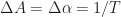
 ) and variable cycle-frequency grid. From top to bottom the block length of the processed data is increased, and the fineness of the grid of visited cycle frequencies is increased in proportion to the increased block length. The two BPSK symbol rates are and .
In each plot, we see at least one prominent feature. For
Cycle-Frequency Resolution in the Context of the Spectral Correlation Function
Let’s consider the time-smoothing method of spectral correlation estimation in discrete time and discrete frequency. The theoretical SCF can be obtained by first averaging over all time, and then increasing the periodogram block length without bound:

where 


(assume 
Now, for the double limit in (33) to hold true, the cyclic periodogram must have a representation of the form
![\displaystyle I_Z^A (m,f) = \left[d_Z(f,\alpha)\otimes S_x^\alpha(f) \right] e^{i2\pi \alpha m Z} + r(f, \alpha, M, m, Z) \hfill (35)](https://s0.wp.com/latex.php?latex=%5Cdisplaystyle+I_Z%5EA+%28m%2Cf%29+%3D+%5Cleft%5Bd_Z%28f%2C%5Calpha%29%5Cotimes+S_x%5E%5Calpha%28f%29+%5Cright%5D+e%5E%7Bi2%5Cpi+%5Calpha+m+Z%7D+%2B+r%28f%2C+%5Calpha%2C+M%2C+m%2C+Z%29+%5Chfill+%2835%29&bg=ffffff&fg=1a1a1a&s=0&c=20201002)
such that

and

But consider two distinct cycle frequencies 


The TSM spectral correlation function estimates for 

![\displaystyle I_Z^A(m,f) = \sum_{k=1}^2 \left[ d_Z(f,\alpha_k) \otimes S_x^{\alpha_k}(f) \right] e^{i2 \pi \alpha_k m Z} + r(f, M, m, T) \hfill (38)](https://s0.wp.com/latex.php?latex=%5Cdisplaystyle+I_Z%5EA%28m%2Cf%29+%3D+%5Csum_%7Bk%3D1%7D%5E2+%5Cleft%5B+d_Z%28f%2C%5Calpha_k%29+%5Cotimes+S_x%5E%7B%5Calpha_k%7D%28f%29+%5Cright%5D+e%5E%7Bi2+%5Cpi+%5Calpha_k+m+Z%7D+%2B+r%28f%2C+M%2C+m%2C+T%29+%5Chfill+%2838%29&bg=ffffff&fg=1a1a1a&s=0&c=20201002)
where

As a check, let’s verify that the double limit holds for
![\displaystyle W(\alpha_1) = \lim_{Z\rightarrow\infty} \lim_{M\rightarrow\infty} \frac{1}{M} \sum_{k=1}^2 \sum_{m=0}^{M-1} \left[ d_Z(f, \alpha_k) \otimes S_x^{\alpha_k}(f) \right] e^{i2\pi\alpha_k m Z} e^{-i2\pi\alpha_1 m Z} \hfill (40)](https://s0.wp.com/latex.php?latex=%5Cdisplaystyle+W%28%5Calpha_1%29+%3D+%5Clim_%7BZ%5Crightarrow%5Cinfty%7D+%5Clim_%7BM%5Crightarrow%5Cinfty%7D+%5Cfrac%7B1%7D%7BM%7D+%5Csum_%7Bk%3D1%7D%5E2+%5Csum_%7Bm%3D0%7D%5E%7BM-1%7D+%5Cleft%5B+d_Z%28f%2C+%5Calpha_k%29+%5Cotimes+S_x%5E%7B%5Calpha_k%7D%28f%29+%5Cright%5D+e%5E%7Bi2%5Cpi%5Calpha_k+m+Z%7D+e%5E%7B-i2%5Cpi%5Calpha_1+m+Z%7D+%5Chfill+%2840%29&bg=ffffff&fg=1a1a1a&s=0&c=20201002)
![\displaystyle = \lim_{Z\rightarrow\infty} \lim_{M\rightarrow\infty} \frac{1}{M} \left( \sum_m \left[d_Z(f,\alpha_1) \otimes S_x^{\alpha_1}(f)\right] e^0 + \sum_m \left[d_Z(f,\alpha_2)\otimes S_x^{\alpha_2}(f)\right] e^{i2\pi(\alpha_2-\alpha_1)mZ} \right) \hfill (41)](https://s0.wp.com/latex.php?latex=%5Cdisplaystyle+%3D+%5Clim_%7BZ%5Crightarrow%5Cinfty%7D+%5Clim_%7BM%5Crightarrow%5Cinfty%7D+%5Cfrac%7B1%7D%7BM%7D+%5Cleft%28+%5Csum_m+%5Cleft%5Bd_Z%28f%2C%5Calpha_1%29+%5Cotimes+S_x%5E%7B%5Calpha_1%7D%28f%29%5Cright%5D+e%5E0+%2B+%5Csum_m+%5Cleft%5Bd_Z%28f%2C%5Calpha_2%29%5Cotimes+S_x%5E%7B%5Calpha_2%7D%28f%29%5Cright%5D+e%5E%7Bi2%5Cpi%28%5Calpha_2-%5Calpha_1%29mZ%7D+%5Cright%29+%5Chfill+%2841%29&bg=ffffff&fg=1a1a1a&s=0&c=20201002)
![\displaystyle = S_x^{\alpha_1}(f) + \lim_{Z\rightarrow\infty} \lim_{M\rightarrow\infty} \sum_{m=0}^{M-1} \frac{1}{M} \left[ d_Z(f,\alpha_2)\otimes S_x^{\alpha_2}(f)\right]e^{i2\pi(\alpha_2-\alpha_1)mZ} \hfill (42)](https://s0.wp.com/latex.php?latex=%5Cdisplaystyle+%3D+S_x%5E%7B%5Calpha_1%7D%28f%29+%2B+%5Clim_%7BZ%5Crightarrow%5Cinfty%7D+%5Clim_%7BM%5Crightarrow%5Cinfty%7D+%5Csum_%7Bm%3D0%7D%5E%7BM-1%7D+%5Cfrac%7B1%7D%7BM%7D+%5Cleft%5B+d_Z%28f%2C%5Calpha_2%29%5Cotimes+S_x%5E%7B%5Calpha_2%7D%28f%29%5Cright%5De%5E%7Bi2%5Cpi%28%5Calpha_2-%5Calpha_1%29mZ%7D+%5Chfill+%2842%29&bg=ffffff&fg=1a1a1a&s=0&c=20201002)
![\displaystyle = S_x^{\alpha_1}(f) + \left(\lim_{Z\rightarrow\infty} \left[d_Z(f,\alpha_2)\otimes S_x^{\alpha_2}(f) \right] \lim_{M\rightarrow\infty}\frac{1}{M} \sum_{m=0}^{M-1} e^{i2\pi(\alpha_2-\alpha_1)mZ} \right) \hfill (43)](https://s0.wp.com/latex.php?latex=%5Cdisplaystyle+%3D+S_x%5E%7B%5Calpha_1%7D%28f%29+%2B+%5Cleft%28%5Clim_%7BZ%5Crightarrow%5Cinfty%7D+%5Cleft%5Bd_Z%28f%2C%5Calpha_2%29%5Cotimes+S_x%5E%7B%5Calpha_2%7D%28f%29+%5Cright%5D+%5Clim_%7BM%5Crightarrow%5Cinfty%7D%5Cfrac%7B1%7D%7BM%7D+%5Csum_%7Bm%3D0%7D%5E%7BM-1%7D+e%5E%7Bi2%5Cpi%28%5Calpha_2-%5Calpha_1%29mZ%7D+%5Cright%29+%5Chfill+%2843%29&bg=ffffff&fg=1a1a1a&s=0&c=20201002)
So, keeping in mind that 
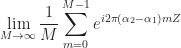
equal to? We recognize this as a geometric series of the form

with 

so that

Therefore,

and by a symmetry argument the same is true for
Now consider the general case where 

![\displaystyle I_Z^A (m,f) = \sum_{k=1}^{N_\alpha} \left[ d_Z(f,\alpha_k) \otimes S_x^{\alpha_k}(f) \right] e^{i2\pi \alpha_k m Z} + r(f, M, m, Z) \hfill (47)](https://s0.wp.com/latex.php?latex=%5Cdisplaystyle+I_Z%5EA+%28m%2Cf%29+%3D+%5Csum_%7Bk%3D1%7D%5E%7BN_%5Calpha%7D+%5Cleft%5B+d_Z%28f%2C%5Calpha_k%29+%5Cotimes+S_x%5E%7B%5Calpha_k%7D%28f%29+%5Cright%5D+e%5E%7Bi2%5Cpi+%5Calpha_k+m+Z%7D+%2B+r%28f%2C+M%2C+m%2C+Z%29+%5Chfill+%2847%29&bg=ffffff&fg=1a1a1a&s=0&c=20201002)
The “noise” term 
![\displaystyle I_Z^A(m,f) = \sum_{k=1}^{N_\alpha} \left[ d_Z(f,\alpha_k) \otimes S_x^{\alpha_k}(f) \right] e^{i2\pi \alpha_k m Z} \hfill (48)](https://s0.wp.com/latex.php?latex=%5Cdisplaystyle+I_Z%5EA%28m%2Cf%29+%3D+%5Csum_%7Bk%3D1%7D%5E%7BN_%5Calpha%7D+%5Cleft%5B+d_Z%28f%2C%5Calpha_k%29+%5Cotimes+S_x%5E%7B%5Calpha_k%7D%28f%29+%5Cright%5D+e%5E%7Bi2%5Cpi+%5Calpha_k+m+Z%7D+%5Chfill+%2848%29&bg=ffffff&fg=1a1a1a&s=0&c=20201002)
or, in terms of the desired spectral correlation estimate

where 
If the combined contributions to 


![\displaystyle \hat{S}_x^\alpha (f) = d_Z(f, \alpha)\otimes S_x^\alpha(f) + \sum_{\alpha_k\neq \alpha} \left[ d_Z(f,\alpha_k) \otimes S_x^{\alpha_k}(f) \right] \frac{1}{M} \sum_{m=0}^{M-1} e^{i2\pi(\alpha_k-\alpha)mZ} \hfill (50)](https://s0.wp.com/latex.php?latex=%5Cdisplaystyle+%5Chat%7BS%7D_x%5E%5Calpha+%28f%29+%3D+d_Z%28f%2C+%5Calpha%29%5Cotimes+S_x%5E%5Calpha%28f%29+%2B+%5Csum_%7B%5Calpha_k%5Cneq+%5Calpha%7D+%5Cleft%5B+d_Z%28f%2C%5Calpha_k%29+%5Cotimes+S_x%5E%7B%5Calpha_k%7D%28f%29+%5Cright%5D+%5Cfrac%7B1%7D%7BM%7D+%5Csum_%7Bm%3D0%7D%5E%7BM-1%7D+e%5E%7Bi2%5Cpi%28%5Calpha_k-%5Calpha%29mZ%7D+%5Chfill+%2850%29&bg=ffffff&fg=1a1a1a&s=0&c=20201002)
The contribution to 
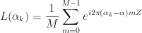
which equals

What is the width of this function? It is approximately 

 from (51). This function reveals that cycle frequencies
  spaced at least
  away from the target cycle frequency contribute relatively little to the spectral correlation function estimate for .
So if this simplified analysis is correct, we once again see that the approximate cycle-frequency resolution for a second-order CSP parameter is the reciprocal of the data-block length used to form the estimate.
Let’s illustrate with some measurements.
First, we repeat the cyclic autocorrelation measurements above with the frequency-smoothing method:
 ) and various cycle-frequency grids. From top to bottom, the grid of visited cycle frequencies becomes finer. The two BPSK symbol rates are and .
 ) and variable cycle-frequency grid. From top to bottom the block length of the processed data is increased, and the fineness of the grid of visited cycle frequencies is increased in proportion to the increased block length. The two BPSK symbol rates are and .
Finally, we apply the strip spectral correlation analyzer to the single-BPSK and two-BPSK cases for various data-block lengths (recall that the two bit rates are
 . Here the grid of visited cycle frequencies is determined by the length of the processed data block .
 and . Here the grid of visited cycle frequencies is determined by the length of the processed data block . Once the block length is such that its reciprocal is less than the difference between the two symbol rates, the algorithm produces two clear peaks near the two true values.
There are multiple dots at the SSCA output locations because the spectral coherence can exceed threshold for multiple values of spectral frequency
We see that once the block length 

Resolution Properties for Second-Order Cyclostationarity: The Take-Away
If you use
Same for the cyclic autocorrelation function.
If you know a cycle frequency
So processing block length and cycle-frequency search grid fineness are inextricably connected.
Resolution Parameters in the Context of Higher-Order Cyclic Cumulants and Cyclic Polyspectra
This topic is advanced–it is much harder to analyze, understand, and illustrate the resolution properties of higher-order cyclic moments, cumulants, and polyspectra. So, we’ll leave it for a future post.
As always, I invite you to leave a comment if you have a question, correction, or relevant experience.
Hi Chad, Thanks for your great blog. It’s been very helpful in developing my own set of cyclostationary analysis tools. One thing I’m confused about is how the parameter choices of the SSCA affects the resolution. For the SSCA, the resolution product is N/Np, which must be >> 1. The cycle frequency resolution is 1/N, and spectral frequency resolution is 1/N_p. Suppose I have a block of N_b=N+N_p input samples. Then how should N and N_p be chosen for blind cyclic frequency detection? I’m using notation from [1]. On the signals I’ve tried, it sometimes seems difficult to get the right combination, especially for OFDM.
I’m also interested in how averaging the SSCA bifrequency plane output for multiple, say K, blocks of N_b samples affects the estimate. Can something similar to Bartlett’s method be said in terms of decreasing the estimator variance by K, but the spectral resolution is also decreased by K? [2] I’ve also observed, on real over-the-air data, that you have to do non-coherent sums in the average.
[1] April, Eric. On the Implementation of the Strip Spectral Correlation Algorithm for Cyclic Spectrum Estimation. In Defence Research Establishment Technical Note 94-2, 1994.
[2] Barbe et al. “Welch Method Revisited: Nonparametric Power Spectrum Estimation Via Circular Overlap” In IEEE Transactions on Signal Processing Feb 2010
Thanks for the thoughtful comment Paul. I attempt responses below.
It seems that you’ve already chosen and
and  through the equation for
  . In general, if you have
  samples, you process those
  samples, which provides the cycle-frequency resolution of
  . You choose the number of channels
  (also called strips) in the SSCA such that
  is as large as possible. This forces you to choose small
  . I’ve found that reliable cycle-frequency estimation can be done in a large number of cases by using a nominal
  of
of  or
or  and using as large a
  as I can.
Real-world OFDM has time-varying cyclostationarity so that the cycle frequencies that you estimate can strongly depend on the particular data block that is processed. For very long blocks, you’ll see similar results for different blocks, but for shorter ones, you might have quite different results block-to-block.
You mean to average the magnitude of the obtained SCF point estimates? You will get a non-coherent averaging gain for sure. Averaging the complex-valued SCF point estimates is more tricky, because the SCF phase depends on how a signal is delayed or advanced. So the averaging could end up destructive.
I’m not sure what you mean here. What real data? I find good results in straightforward application of the SSCA, FSM, and TSM to various kinds of captured communication signals such as WCDMA, LTE, CDMA, EVDO, ATSC-DTV. However, if the signal is bursty, and the bursts have random start times, then using a long data block containing multiple bursts can result in a small SCF due to the same kind of destructive interference I mentioned above. You essentially have multiple versions of the signal within the data block, and each has a different start time relative to the time origin. So short-block incoherent averaging has to be done here, or somehow the bursts have to be individually detected and aligned prior to CSP (not attractive).
Hi chad, .
.
In figure 9 we look at the CAF maxima, i.e.
How do we find this maximum? Using a grid of Tau? If so, is there a resolution issue here as well?
Sure, in the same way you would maximize the magnitude of any discrete-time sequence. For the autocorrelation or cyclic autocorrelation, most estimation methods I know will naturally produce estimates on a set of that has spacing equal to the spacing between successive input samples for the data to be processed (that is, the spacing is the sampling incrementt).
Always! This is a resolution-in-time problem. It comes up quite forcefully in things like time-delay estimation.
You can employ elementary signal-processing methods to improve the resolution, such as interpolation and increasing the sampling rate. Generally speaking this particular resolution problem is not as important in CSP as the resolutions in frequency and cycle frequency.