
In this short post, I describe some errors that are produced by MATLAB’s strip spectral correlation analyzer function commP25ssca.m. I don’t recommend that you use it; far better to create your own function.
If you subscribe to MATLAB’s Communication Toolbox, you have access to an implementation of the SSCA: commP25ssca.m. The function has help text that looks like this:
This function is written according to (1) Figure 3 and Figure 5 of the
reference: E. L. Da Costa, “Detection and Identification of
Cyclostationary Signals”. MS Thesis. 1996. (2) Section 3.2 of the
reference: Eric April, “On the Implementation of the Strip Spectral
Correlation Algorithm for Cyclic Spectrum Estimation”. February, 1994.
The function takes four arguments:
function [Sx,alphao,fo] = commP25ssca(input,fs,df,dalpha)
where input is the complex-valued input data, fs is the sampling rate corresponding to input, df is the spectral resolution, and dalpha is the cycle-frequency resolution.
commP25ssca.m computes the non-conjugate spectral correlation function (SCF). So if you want the conjugate spectral correlation or either of the coherences, you’ll have to write your own functions or modify commP25ssca.m.
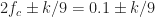
The trouble is that this function produces strong spurious cycle frequencies. In particular, it produces large spectral correlation function magnitudes for the normalized cycle frequencies of 
I consider two inputs. The first is a slight variation of our old friend the rectangular-pulse BPSK signal. In this variation, the bit rate is 


I use two implementations of the SSCA. The first is commP25ssca.m and the second is one that I’ve written myself. The latter has been validated by checking its output against the theoretical spectral correlation function for several signals for which we have nice formulas for the SCF (such as PSK and QAM).
For my SSCA implementation, I run with 


Here are the results for the rectangular-pulse BPSK signal:


And here are the results for WGN:


You can see that commP25ssca.m produces the false cycle frequencies of 


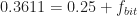
The set of spurious cycle frequencies depends on the input parameter df. I’ve not done any kind of comprehensive study of this problem, but here is the graph of the commP25ssca.m output when we modify df from 

I haven’t tried to figure out what is going wrong with commP25ssca.m. If you do, please go ahead and post your findings to the comments section of this post.
I want to thank reader Serg for bringing this MATLAB problem to my attention!
Hi Dr. Spooner,
1st Thank you so much for this very helpful blog. For one thing I’d have never known about the defect in the Matlab code if you hadn’t posted about it. I had based my C++ implementation off of it and the papers by Nancy Carter and da Costa.
2.) I’m pretty sure it is result of the replication process that is prevalent in those papers. The reason I believe this to be the case is Eric April references it in his paper on the Strip Spectral Correlation Algorithm (section 3.1, just before section 3.2) and says it causes this exact problem. I’ve spent about 2 weeks trying to figure this out and haven’t had a chance to verify yet. For one thing I’m curious how you deal with complex demodulates being at the full rate, since x(t) has been decimated by L.
3.) Also I’m unsure if there is one windowing function or two? April seems to indicate there are 2 but most papers seem to have just one. Although, most of the equations have an a(n) and g(n).
Thank You.
Thanks for the comments, Zack, and for stopping by the CSP Blog.
I’ll answer (2) in reply to another of your comments.
Regarding (3), yes there are two windowing functions in the normal SSCA estimator expression: and
and  . The former is a window applied to the short-time FFTs that comprise the front-end “channelizer” function of the SSCA, and the latter is a window applied to the long-time FFTs that comprise the back-end “strip” function of the SSCA. In my implementations,
  is a Dolph-Chebyshev window and
  is just a rectangle (no windowing). I’ve not been able to squeeze out enough performance gain for the cost of a non-rectangular
  .
.
Sorry, I was wrong. It isn’t the replication, it is the decimation by L in the channelizer (which necessitates the replication). If you modify commP25ssca to set L = 1 the false cycle frequencies disappear. However, apparently Brown suggested this as a way of lowering computational costs. April suggests this might be worthwhile as the false cycles could be predicted. Any suggestions?
Ah, good. Long ago I abandoned in the SSCA. It is not hard to simply store all the front-end channelizer-FFT coefficients and then use them in each back-end strip FFT. My position is
  is useful in memory-limited situations. But then I suppose you pay a bit of a price in false cycle frequencies. None of my machines are particularly low on memory these days…
I suppose commP25ssca should have as an input variable.
Do you use “replication” here to mean “interpolation?”
I forgot to ask, do you truly get no correlation w/ WGN in your ssca’s? If so do you do something special? As far as I can tell L > 1 is the only thing “wrong” with the Matlab code, and it doesn’t seem to effect this .I even tried the Dolph-Chebyshev filter and didn’t notice much of a difference.
Thanks
Well, certainly not for every WGN input, no. There will inevitably be some false alarms. But yes, in the plots I provided, I detected no CFs using the coherence when WGN was at the input.
You might want to put some “keep out” zones in your SSCA and FAM code, so that CFs that are too small are rejected. Small non-conjugate CFs are associated with SCF slices very near the PSD, and so are contaminated with cycle leakage, which can inflate the coherence.
Chad, has the SSCA been found useful for blind mixed communication signal detection? In particular, for a mixed signal situation where one signal, e.g., QPSK, has a wide enough bandwidth that encompasses several other comm signals, e.g., 8PSK, 16QAM, of equal or lower amplitudes and smaller bandwidths?
Yes! You might want to check out the post on signal selectivity.
The SSCA, and the FAM, and much less efficiently the FSM-in-a-loop and TSM-in-a-loop, can produce the cycle frequencies of multiple cochannel signals, regardless of their relative bandwidths. The amount of data that you need to process to get accurate and reliable results will, however, depend on the bandwidths of the signals. In other words, if you have a 10 MHz signal and a cochannel signal has bandwidth 10 kHz, then for any processed data-block length, you’ll have about 1000 fewer symbols for the narrow signal to average over in your estimator.
Here is an example. I added three narrowband signals, BPSK, 8PSK, and 16QAM, to a relatively wideband QPSK signal:
QPSK: symbol rate = 0.5, carrier = 0
BPSK: symbol rate = 0.04, carrier = -0.3
8PSK: symbol rate = 0.0208, carrier = 0.05
16QAM: symbol rate = 0.067, carrier = 0.27
If I process a block of data corresponding to that scene with the SSCA, and also perform coherence-based cycle-frequency detection, I get a cyclic domain profile that looks like this:
However, much more CSP needs to be done to take the next steps toward modulation classification. The SSCA is useful, but not sufficient to perform a full analysis. It quickly gets you in the right ballpark, though, and you can construct algorithms that parse those cyclic domain profiles, compute cyclic cumulants, perform joint signal classification and parameter estimation, etc.
You could also choose to extract narrowband slices of the data in the PSD above, and subject each one to an SSCA analysis and modulation-recognition algorithms.
Does that help?
Thank you, Chad. Yes, this helps. I initially started with EEMB/ICA with clustering of mixed signals into only a single antenna. With two or more antennas…no problem but I don’t get such luxury. Consequently, I wondered about SSCA and your response appears what I may need to detection of whether or not a mixed signal scenario exists. As far as the modulation classification, as I mentioned in an earlier post, cyclic complex HOCs worked very well down to SNR = 4dB so long as I took care of the non-integer sampling with polyphase filters.
Yeah, I usually don’t have more than one sensor either…
Glad to hear my tip might help!
For other readers of this thread, there is no intrinsic SNR floor or wall when performing detection or modulation recognition with cyclic cumulants (of any order, including two). If you fix the scenario, the sampling rate, and the number of samples you are willing to process, then there is a minimum SNR for which you can obtain adequate performance. To do well at lower SNR requires processing longer data blocks. See the post on the cycle detectors (admittedly not blind processing) to see how performance improves with block length for each SNR considered. And also the post on the resolution product.
Your comment about needing additional CSP to also encompass modulation classification is correct. I have been looking into cyclic moments and cyclic cumulants to proceed forward (after success with blind modulation classification using HOCs for single signals from a single antenna) for blind mixed signal detection/classification.
In so doing, I came across a dissertation in which the author was focused on cyclic moments for mixed signal detection and modulation classification rather than cyclic cumulants. The dissertation title is, “Mixed Signal Detection, Estimation, and Modulation Classification,” out of Wright State University and cites several of your papers (https://corescholar.libraries.wright.edu/cgi/viewcontent.cgi?article=3404&context=etd_all). It doesn’t appear that the author makes use of SCF and thus no mention of SSCA; only cyclic moment analysis.
Would like to get your thoughts of this paper, in light of your work, as a process towards blind mixed signal detection/classification.
I gave many hours of my time to the author of that dissertation, Yang Qu, a couple years back, and even visited him and his advisor once at Wright State in Ohio.
You can find quite a few comments on the CSP Blog from Yang. He gives me a shout-out in his dissertation Acknowledgement, but I wasn’t on the committee.
I do think he attempted extensive use of cyclic cumulants in the dissertation:
(page 60) and the basic idea is similar to what I have published and have advocated on the CSP Blog: Use second-order processing (temporal or spectral moments) and selective fourth-order processing (temporal moments) to estimate basic parameters like symbol rates and carrier frequency offsets. Then use those to determine the cycle-frequency pattern exhibited by the signal, and finally use cyclic cumulants to create good classification features.
The dissertation is a bit hard to follow, and there are lots of mysterious and, frankly, wrong-looking plots throughout. So if you give it more than a skim, beware. I hate to have to say that, but I don’t want to mislead you.