Frequency Shift (FRESH) Filtering for Single-Sensor Cochannel Signal Separation

CSP can be used to separate cochannel contemporaneous signals. The involved signal-processing structure is linear but periodically time-varying.

In most of the posts on the CSP Blog we’ve applied the theory and tools of CSP to parameter estimation of one sort or another: cycle-frequency estimation, time-delay estimation, synchronization-parameter estimation, and of course estimation of the spectral correlation, spectral coherence, cyclic cumulant, and cyclic polyspectral functions.

In this post, we’ll switch gears a bit and look at the problem of waveform estimation. This comes up in two situations for me: single-sensor processing and array (multi-sensor) processing. At some point, I’ll write a post on array processing for waveform estimation (using, say, the SCORE algorithm The Literature [R102]), but here we restrict our attention to the case of waveform estimation using only a single sensor (a single antenna connected to a single receiver). We just have one observed sampled waveform to work with. There are also waveform estimation methods that are multi-sensor but not typically referred to as array processing, such as the blind source separation problem in acoustic scene analysis, which is often solved by principal component analysis (PCA), independent component analysis (ICA), and their variants.

The signal model consists of the noisy sum of two or more modulated waveforms that overlap in both time and frequency. If the signals do not overlap in time, then we can separate them by time gating, and if they do not overlap in frequency, we can separate them using linear time-invariant systems (filters).

Relevant FRESH filtering publications include My Papers [45, 46] and The Literature [R6].

Motivating Example

Let’s first illustrate the problem using a concrete example.

Our signal model consists of a desired signal $d(t)$ , noise $n(t)$ , and interference $i(t)$ ,

$\displaystyle x(t) = d(t) + i(t) + n(t), \hfill (1)$

where the interference $i(t)$ may be zero (no interference) or the sum of multiple distinct statistically independent interference signals $i_j(t)$ , for $j = 1, 2, \ldots, N_I$ . In our motivating example, we use $N_I = 2$ , and the signal of interest $d(t)$ and the interferers are all BPSK signals. Estimated power spectra for the individual signals and their noisy sum are shown in Figure 1.

Figure 1. Power spectra for the signal of interest (black), the two interferers (cyan and blue), and their noisy sum (red). Note that this is a hard example in that there are no frequency components for the signal of interest that are not interfered with by a frequency component from one of the interferers.

We’ll use the setup in Figure 1 throughout the post to unify the exposition. All frequencies and times in this post are normalized by the sampling rate, as is the custom at the CSP Blog, which is equivalent to using a sampling rate of unity. The parameters of each of the involved signals are shown in Table 1.

Signal Name	Parameter Name	Parameter Value	Parameter Units
Signal of Interest	Modulation Type	BPSK
	Power	0	dB
	Bit Rate	1/5	Hz
	Carrier Offset	-0.01	Hz
	Pulse Type	SRRC
	Excess Bandwidth	0.5
Interferer 1	Modulation Type	BPSK
	Power	-10	dB
	Bit Rate	1/6	Hz
	Carrier Offset	0.13	Hz
	Pulse Type	SRRC
	Excess Bandwidth	0.5
Interferer 2	Modulation Type	BPSK
	Power	4
	Bit Rate	1/7
	Carrier Offset	-0.08
	Pulse Type	SRRC
	Excess Bandwidth	0.5
Noise	Type	AWGN
	Power	-20	dB

Table 1. Parameter values for the signals used in the running example for this FRESH-filtering post.

The goal of a FRESH filter is to process the received noisy interference-corrupted data and return a signal that has the interference attenuated as much as possible, while maintaining the amplitude of the signal of interest. (We can always reduce the interference to zero by just multiplying the whole input data signal by zero, but that also annihilates the signal of interest.) In particular, if the interference is so bad that we cannot successfully demodulate the signal of interest, can we use a FRESH filter to bring the interference level down enough to permit demodulation?

To measure how much interference and noise is present in the input or output of a FRESH filter, or any other signal-separation system, we will use the normalized mean-squared error (NMSE) expressed in decibels (dB). For the model (1), the NMSE is given by

$\displaystyle E = \frac{1}{P_d} \left[ \frac{1}{N} \sum_{t=0}^{N-1} |x(t) - d(t)|^2 \right] \hfill (2)$

where $P_d$ is the power (variance) of $d(t)$ . The quantity in the square brackets in (2) is the mean (average) squared error between $x(t)$ and the desired signal $d(t)$ , and the NMSE expresses this as a fraction of the power of $d(t)$ . Moreover, we convert that value to decibels by

$\displaystyle E_{dB} = 10\log_{10}(E) \hfill (3)$

For our motivating example in Figure 1, the NMSE is about 4.2 dB. That means the ratio of the total power of the interference and noise to the signal power is about 2.6. So think of the NMSE as the reciprocal of an SNR–higher is worse, lower is better. If the NMSE is -10 dB, then the total noise and interference power corrupting the signal is ten times less than the signal power–the SNR is about +10 dB.

That’s the motivating example. How do we separate the signal from the cochannel interference and noise? That depends on what kind of processing we are willing to apply. As usual in such situations, let’s start with a linear time-invariant system–a filter.

An Optimal LTI Solution: Wiener Filtering

One way to approach the signal-separation problem is to specify the form of the processing and then attempt to find the optimal version of that form. When the form is restricted to a linear time-invariant system, or filter, the resulting optimal form is called the Wiener filter, when the criterion for optimality is to minimize the mean-squared error.

The Wiener filter has transfer function given by

$\displaystyle H_w(f) = \frac{S_{dx}(f)}{S_x(f)} \hfill (4)$

where $S_{dx}(f)$ is the cross spectral density between the desired signal $d(t)$ and the received signal $x(t)$ and $S_x(f)$ is the spectral density of the received signal.

Does the filter in (4) make physical sense? Let’s try to check. Suppose $i(t)$ is zero so that we just have $x(t) = d(t) + n(t)$ . Then $S_{dx}(f) = S_d(f)$ because $d(t)$ and $n(t)$ are uncorrelated, and $S_x(f) = S_d(f) + S_n(f)$ . The Wiener filter is

$H_w(f) = \frac{S_d(f)}{S_d(f) + S_n(f)} \hfill (5)$

For those frequencies for which $S_d(f) = 0$ , the filter transfer function is zero, indicating that the filter should not pass any frequency components that do not contain any of the desired signal–the transfer function is ideally zero. For those frequency components for which $S_d(f) \ll S_n(f)$ , the transfer function is approximately $H_w(f) \approx S_d(f)/S_n(f) \ll 1$ , so that these frequency components are attenuated. For those components such that $S_d(f) \gg S_n(f)$ , the filter is approximately $H_w(f) \approx 1$ , indicating that the filter should just pass those frequency components mostly unchanged. In other words, the filter attenuates the input in frequency bands where the noise is dominant (in terms of power) and passes unchanged those components where the signal is dominant. Makes sense, right?

Now add back in the interference. Suppose the interference $i(t)$ has a bandwidth that is much narrower than the bandwidth of $d(t)$ , but is cochannel with $d(t)$ . The filter is, in general,

$H_w(f) = \frac{S_d(f)}{S_d(f) +S_i(f) +S_n(f)}, \hfill (6)$

and notice that for those frequencies $f$ for which $S_i(f)$ is not zero, the transfer function is attenuated because $S_d(f) + S_i(f) + S_n(f) > S_d(f) + S_n(f)$ . Suppose $S_i(f)$ is very large compared to $S_d(f)$ and $S_n(f)$ for some frequency $f$ . Then for that frequency, $H_w(f) \ll 1$ , and the filter severely attenuates the input signal. So we see that the Wiener filter has all-pass filter, notch filter, or bandpass filter characteristics over frequency as needed in response to the spectral characteristics of the noise and interference relative to those for the signal of interest.

But … what about when the functions $S_d(f)$ and $S_i(f)$ are similar? Let’s say that $S_i(f) = S_d(f)$ . Then

$\displaystyle H_w(f) = \frac{S_d(f)}{2S_d(f) + S_n(f)} \hfill (7)$

When the SNR is not low, $2S_d(f) \gg S_n(f)$ over those frequencies for which $S_d(f)$ is not small, and we have

$\displaystyle H_w(f) \approx \frac{S_d(f)}{2S_d(f)} = 1/2 \hfill(8)$

So that all frequency components–signal and interferer–are passed without any relative attenuation. That is, the NMSE of the output is the same as the NMSE at the input, neglecting the slight decrease obtained due to filtering the out-of-band noise components.

When the interferer(s) substantially spectrally overlaps the signal of interest, and the interferer and signal have similar bandwidths and power levels, the optimal linear time-invariant signal-separation system [Wiener filter] is ineffective.

Let’s get quantitative and apply the Wiener filter to our motivating example in Figure 1. We use the FSM to estimate the power spectra needed to form the filter’s transfer function in (5). To form the impulse-response function for the filter, we simply inverse transform the obtained transfer function and retain only the 128 values in the energetic central portion near $\tau = 0$ . The result is an impulse-response function for a finite impulse response (FIR) filter, which we apply to the data $x(t)$ . We then synchronize to the filter output, scale it (why?), and compute the NMSE. The result is an NMSE of -0.2 dB and the power spectrum of the input and output are shown in Figure 2.

Figure 2. Input and output spectra for the application of the Wiener filter to the motivating example in Figure 1 and Table 1. The input NMSE is 4.2 dB and the output NMSE is -0.2 dB, for an overall gain of 4.4 dB.

The Wiener filter computed by my software, applied to obtain the signal corresponding to the green line in Figure 2, has transfer function shown in Figure 3.

Figure 3. Transfer function for the Wiener filter computed by my FRESH filtering software (rather than by numerical evaluation of theoretical auto- and cross-spectral densities) for the situation shown in Figure 1. Note the shape of the transfer function over the bandwidth of the signal of interest (about [-0.15, 0.125]). The filter strongly attenuates the frequency components where the interferer is strongest ([-0.15, 0]), mildly attenuates the frequency components where the interference is weak ([0, 0.125]), and very strongly attenuates the frequency components outside the signal band.

A typical desired output SINR needed for adequate demodulation performance is something around 6 dB. So we see that the Wiener filter cannot separate the signals adequately in this particular case. So we need something else. Since the linear time-invariant system is ineffective, we can consider nonlinear time-invariant systems, nonlinear time-variant systems, or linear time-variant systems. In particular, we can consider linear time-variant systems where the time variation is periodic (surprised?): linear periodically time-variant filtering.

Linear Periodically Time-Variant Filtering

To fully understand FRESH filtering, I recommend starting with The Literature [R6] and W. A. Brown’s doctoral dissertation. I’ll sketch my understanding of linear periodically time-variant (LPTV) filtering and FRESH filtering here, following closely The Literature [R6].

As we know well, a linear time-invariant system is characterized by the impulse-response function $h(t)$ , which relates the system input $x(t)$ to the system output $y(t)$ through the convolution

$\displaystyle y(t) = \int_{-\infty}^\infty h(t-u)x(u)\, du. \hfill (9)$

For a linear time-varying system, the impulse response is now a general function of time and delay, so that $h(t-u)$ is replaced by $h(t,u)$ ,

$\displaystyle \int_{-\infty}^\infty h(t,u) x(u)\, du \hfill (10)$

For a linear periodically (or almost periodically) time-varying system, the form of that general impulse response is constrained to be representable by a generalized Fourier series,

$\displaystyle h(t,u) = \sum_{\gamma} h_\gamma(t-u)e^{i 2 \pi \gamma u} \hfill (11)$

where the $h_\gamma(\tau)$ functions are obtained by an infinite-time version of the usual Fourier-series coefficient formula,

$\displaystyle h_\gamma(\tau) = \lim_{T\rightarrow\infty} \frac{1}{T} \int_{-T/2}^{T/2} h(t+\tau,t) e^{-i2\pi \gamma t} \, dt \hfill (12)$

Putting (11) together with (10), we have the input-output relation for a general linear periodically time-varying system

$\displaystyle y(t) = \sum_\gamma \int_{-\infty}^\infty h_\gamma(t-u)e^{i 2 \pi \gamma u} x(u) \, du \hfill (13)$

Now associate the complex exponential with the input $x(u)$ to yield

$\displaystyle y(t) = \sum_\gamma h_\gamma(t) \otimes [x(t)e^{i 2 \pi \gamma t}] \hfill (14)$

which is a sum of filtered frequency-shifted versions of the input: FREquency-SHift (FRESH) filtering.

A final wrinkle involves whether the input $x(t)$ is real-valued or complex-valued. It turns out we need to filter the complex envelope and its conjugate, unlike the case of linear time-invariant filtering, where we can always just apply a filter to the complex envelope, ignoring its conjugate. For the full story, see Brown’s dissertation. I’ll give a justification here.

Suppose we have real-valued signals $x(t)$ and $y(t)$ related by a convolution,

$\displaystyle y(t) = \int_{-\infty}^\infty h(t-u)x(u)\, du. \hfill (15)$

How is the analytic signal of $y(t)$ related to the analytic signal of $x(t)$ and the filter $h(t)$ ? The analytic signal for $x(t)$ is the positive-frequency portion of the signal, $2u(f)X(f)$ . It can be obtained by convolving with the following impulse response function

$\displaystyle h_{AS}(t) = \delta(t) + j/(\pi t). \hfill (16)$

That is, using our normal CSP-Blog Fourier transform notation,

$\displaystyle x_{AS}(t) = x(t) \otimes h_{AS}(t) \Longleftrightarrow 2u(f)X(f). \hfill (17)$

Now, what is $y_{AS}(t)$ ? Let’s take it step by step,

$\displaystyle y_{AS}(t) = y(t) \otimes h_{AS}(t) = \left[\int_{-\infty}^\infty h(t-u)x(u)\,du \right] \otimes h_{AS}(t) \hfill (18)$

$\displaystyle = \int_{-\infty}^\infty h_{AS}(t-v) \left[\int_{-\infty}^\infty h(v-u)x(u)\, du \right] \, dv \hfill (19)$

$\displaystyle = \int_{-\infty}^\infty h_{AS}(t-u-w) \int_{-\infty}^\infty h(w) x(u) \, dw \, du \hfill (20)$

$\displaystyle = \int_{-\infty}^\infty \int_{-\infty}^\infty h(w) \left[h_{AS}(t-u-w)x(u) \, du \right] \, dw \hfill (21)$

$\displaystyle = \int_{-\infty}^\infty h(w) \left[ \int_{-\infty}^\infty h_{AS}([t-w] - u) x(u)\, du \right] \, dw \hfill (22)$

$\displaystyle = \int_{-\infty}^\infty h(w) x_{AS}(t-w) \, dw \hfill (23)$

$\displaystyle = x_{AS}(t) \otimes h(t). \hfill (24)$

We see that the analytic signal for $y(t)$ can be obtained by filtering the analytic signal for $x(t)$ using the same filter as was applied to the real-valued signals. The complex envelope is a filtered and shifted version of the analytic signal, so we can conclude that filtering a bandpass real-valued signal is equivalent to filtering its complex envelope. You need to make sure you convert the bandpass filter for the real signal (and analytic signal) to a lowpass filter once you have obtained the complex envelope.

In the case of linear time-invariant filtering, then, filtering can be performed using the complex envelope and we’ll get what we would have gotten had we processed the real-valued bandpass signal.

What about when the processing is not linear time-invariant processing? In particular, we know we’re interested in linear time-varying processing. Let’s look at that case now.

The input-output relationship between real-valued $x(t)$ and $y(t)$ is now given by

$\displaystyle y(t) = \int_{-\infty}^\infty h(t,u) x(u) \, du \hfill (25)$

which is not a convolution unless $h(t,u) = h(t-u)$ as in the previous analysis. Proceeding as before, let’s look at the analytic signal for $y(t)$ . What is it in terms of the analytic signal for $x(t)$ now that we have a time-varying system?

$\displaystyle y_{AS}(t) = y(t)\otimes h_{AS}(t) = \left[ \int_{-\infty}^\infty h(t,u) x(u)\, du \right] \otimes h_{AS}(t) \hfill (26)$

$\displaystyle = \int_{-\infty}^\infty \int_{-\infty}^\infty h(t-v, u) x(u) h_{AS}(v) \, du\, dv \hfill (27)$

We need to express $x(t)$ in terms of its analytic signal $x_{AS}(t)$ . We start by writing what we know,

$\displaystyle x_{AS}(t) \Longleftrightarrow 2u(f)X(f) \hfill (28)$

where

$\displaystyle x(t) \Longleftrightarrow X(f) \hfill (29)$

and $u(t)$ is the unit-step function, which is equal to zero for $t < 0$ and one otherwise. Because $x(t)$ is real-valued, its Fourier transform possesses conjugate symmetry,

$\displaystyle X(f) = X^*(-f) \hfill (30)$

and so we can express the transform of $x(t)$ as the sum of a positive-frequency term and a negative-frequency term as follows

$\displaystyle x(t) \Longleftrightarrow u(f) X(f) + u(-f)X^*(-f) \hfill (31)$

Here we are neglecting a complication that occurs when $X(0)$ is not zero; let’s assume it is, which is reasonable for $x(t)$ being an RF (bandpass) signal.

Equation (31) implies the following formulation of the real-valued signal $x(t)$ in terms of its analytic signal

$\displaystyle x(t) = \frac{1}{2} (x_{AS}(t) + x^*_{AS}(t)) \hfill (32)$

because

$\displaystyle x_{AS}(t) \Longleftrightarrow 2u(f)X(f) \Rightarrow x^*_{AS}(t) \Longleftrightarrow 2u(-f)X^*(-f) \hfill (33)$

Substituting our expression involving the analytic signal into (27) gives

$\displaystyle y_{AS}(t) = \int_{-\infty}^\infty \int_{-\infty}^\infty h(t-v, u) h_{AS}(v) \frac{1}{2} \left[ x_{AS}(u) + x^*_{AS}(u)\right] \, du \, dv \hfill (34)$

$\displaystyle y_{AS}(t) = \frac{1}{2} \int\int h(t-v,u)h_{AS}(v)x_{AS}(u) \, du\, dv + \frac{1}{2} \int\int h(t-v, u)h_{AS}(v) x^*_{AS}(u)\, du\, dv \hfill (35)$

which means to get the analytic signal for $y(t)$ requires that we filter both the analytic signal for $x(t)$ and its conjugate. It follows that if we are working with complex envelopes in a linear periodically time-varying system (FRESH filter), we need to separately filter the complex envelope and its conjugate and combine the results. The final structure, then, that we are discussing in this post is the FRESH filter for complex signals:

$\displaystyle y(t) = \sum_{m=1}^M a_m(t) \otimes [x(t)e^{i2\pi \alpha_m t}]+\sum_{n=1}^N b_n(t) \otimes [x^*(t) e^{i 2 \pi \beta_n t}], \hfill (36)$

where $a_m(t)$ are the non-conjugate filters, $\alpha_m$ are the non-conjugate frequency shifts, $b_n(t)$ are the conjugate filters, $\beta_n$ are the conjugate frequency shifts, and $M$ and $N$ can be infinite.

Optimal Linear Periodically Time-Variant Filtering: The Cyclic Wiener Filter

The signal-processing structure that we want to investigate is (36), the FRESH filter, which is a linear (almost) periodically time-variant system. It accepts a single complex-valued input that contains two or more temporally and spectrally overlapping cyclostationary signals, and aims to produce a single complex-valued output that is a high-SINR version of just one of the signals in the input. That is, it performs signal separation through waveform estimation.

The engineering question is: How do we choose the frequency shifts $\{\alpha_m\}$ and $\{\beta_n\}$ and the associated impulse-response functions $\{a_m(t)\}$ and $\{b_n(t)\}$ ?

To proceed, The Literature [R6] keeps the FRESH structure generic–we don’t specify the shifts, which is equivalent to keeping the kernel $h(t,u)$ generic, and attempt, a la Wiener, to minimize the error between the system output and the desired signal in the input. This leads to a set of constraints on the filters that involve the frequency shifts. I call these the FRESH-filtering design equations, and they are (16a) and (16b) in [R6], and (37)-(38) here:

$\displaystyle \sum_{m=1}^M S_x^{\alpha_k - \alpha_m} \left( f - \frac{\alpha_m - \alpha_k}{2} \right) A_m(f)$

$\displaystyle + \sum_{n=1}^N S_{xx^*}^{\beta_n - \alpha_k} \left(f-\frac{\beta_n+\alpha_k}{2}\right)^* B_n(f) = S_{dx}^{\alpha_k} \left(f - \frac{\alpha_k}{2}\right), \hfill (37)$

where $k$ ranges from $1$ to $M$ , and

$\displaystyle \sum_{m=1}^M S_{xx^*}^{\beta_k - \alpha_m} \left(f - \frac{\alpha_m - \beta_k}{2}\right) A_m(f)$

$\displaystyle + \sum_{n=1}^N S_x^{\beta_k - \beta_n} \left(-f + \frac{\beta_n + \beta_k}{2} \right) B_n(f) = S_{dx^*}^{\beta_k} \left(f - \frac{\beta_k}{2}\right), \hfill (38)$

where $k$ ranges from $1$ to $N$ .

There are a couple things to notice about the design equations and some terminology to introduce to help us understand experimental results (outputs of a software system aimed at implementing (37)-(38)).

First, notice that on the left-hand sides, two kinds of non-conjugate spectral correlation function appear: one that involves differences between the non-conjugate frequency shifts $\alpha_k$ and one that involves differences between the conjugate frequency shifts $\beta_k$ .

Second, notice that on the left-hand sides, two kinds of conjugate spectral correlation function appear: one that involves $\beta_n - \alpha_k$ and the other that involves $\beta_k - \alpha_m$ . In both cases, the conjugate spectral correlation function is evaluated for a cycle frequency that is a mixture of non-conjugate and conjugate FRESH-filter frequency shifts. We’ll call the first set of cycle frequencies ‘Mixture 1‘ and the second ‘Mixture 2,’ although they are really the same set, I want to be sure that we are enumerating them properly, and estimating the conjugate spectral correlation functions properly, separately because of the complexity and trickiness of implementing the design equations.

The mathematical problem is to solve (37)-(38) for the $A_m(f)$ and $B_n(f)$ given two sets of frequency shifts $\{\alpha_m\}_{m=1}^M$ and $\{\beta_n\}_{n=1}^N$ .

A secondary, and vexing, problem is how to choose the frequency-shift sets. The design equations, if solved, will provide the filters $A_m(f)$ and $B_n(f)$ that minimize the mean-squared error between FRESH output and the desired signal, but that minimum error will vary with the selection of the frequency shifts.

There is some optimal set of frequency shifts, possibly infinite in size, that provides the smallest minimum mean-squared error. For this set of frequency shifts, and the filters corresponding to the solution of the design equations for those shifts, the corresponding FRESH filter is called the cyclic Wiener filter. For all other sets of shifts, we just have some suboptimal (non-cyclic-Wiener) FRESH filter, which of course may be quite good.

In the remainder of this post, we’ll look at various selections of the frequency shifts for our motivating problem and variants, we’ll discuss how to solve the design equations, and we’ll introduce adaptive FRESH filtering.

Constrained Optimal FRESH Filtering (FRESH Filtering in Practice)

Solving the Design Equations

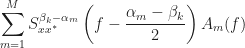
The way I solve the design equations (37)-(38) is one frequency $f$ at a time using simple linear algebra. We can write (37) more explicitly in terms of the filter transfer functions $A_m(f)$ and $B_n(f)$ , again thinking of the equations as involving only a single value of $f$ in the following way

$\displaystyle S_x^{\alpha_k-\alpha_1}\left(f-\frac{\alpha_1+\alpha_k}{2}\right) A_1(f) + \ldots + S_x^{\alpha_k-\alpha_M}\left(f-\frac{\alpha_M+\alpha_k}{2}\right)A_m(f)$

$\displaystyle + S_{xx^*}^{\beta_1-\alpha_k}\left(f - \frac{\beta_1+\alpha_k}{2}\right) B_1(f) + \ldots + S_{xx^*}^{\beta_N-\alpha_k}\left(f - \frac{\beta_N+\alpha_k}{2}\right) B_N(f)$

$\displaystyle = S_{dx}^{\alpha_k}(f - \frac{\alpha_k}{2}) \hfill (39)$

And a similar expression exists for the long form of (38). We can write the two sets of equations as a single set of linear equations in the unknown filter transfer functions by defining the following vectors and matrix,

$\displaystyle \mathbf{B}(f) = [S_{dx}^{\alpha_1}(f - \frac{\alpha_1}{2}) \ldots S_{dx}^{\alpha_M}(f-\frac{\alpha_M}{2}) \ S_{dx^*}^{\beta_1}(f - \frac{\beta_1}{2}) \ldots S_{dx^*}^{\beta_N}(f - \frac{\beta_N}{2})]^\top \hfill (40)$

$\displaystyle \mathbf{H}(f) = [A_1(f) \ldots A_M(f) \ B_1(f) \ldots B_N(f)]^\top \hfill (41)$

$\displaystyle \mathbf{S}(f) = \begin{pmatrix} S_x^{\alpha_1-\alpha_1}(f-\frac{\alpha_1+\alpha_1}{2}) & \hdots & S_x^{\alpha_1-\alpha_M}(f - \frac{\alpha_1-\alpha_M}{2}) & S_{xx^*}^{\beta_1-\alpha_1}(f-\frac{\beta_1+\alpha_1}{2}) & \hdots & S_{xx^*}^{\beta_N-\alpha_1}(f-\frac{\beta_N+\alpha_1}{2}) \\ S_x^{\alpha_2-\alpha_1}(f-\frac{\alpha_2+\alpha_1}{2}) & \hdots & S_x^{\alpha_2-\alpha_M}(f-\frac{\alpha_2-\alpha_M}{2}) & S_{xx^*}^{\beta_1-\alpha_2}(f-\frac{\beta_1+\alpha_2}{2}) & \hdots & S_{xx^*}^{\beta_N-\alpha_2}(f-\frac{\beta_N+\alpha_2}{2}) \\ \vdots & \vdots & \vdots & \vdots & \vdots & \vdots \\ S_x^{\alpha_M-\alpha_1}(f-\frac{\alpha_M+\alpha_1}{2}) & \hdots & S_x^{\alpha_M-\alpha_M}(f-\frac{\alpha_M-\alpha_M}{2}) & S_{xx^*}^{\beta_1-\alpha_M}(f-\frac{\beta_1+\alpha_M}{2}) & \hdots & S_{xx^*}^{\beta_N-\alpha_M}(f-\frac{\beta_N+\alpha_M}{2}) \\ S_{xx^*}^{\beta_1-\alpha_1}(f-\frac{\alpha_1+\beta_1}{2}) & \hdots & S_{xx^*}^{\beta_1-\alpha_M}(f-\frac{\alpha_M+\beta_1}{2}) & S_x^{\beta_1-\beta_1}(-f+\frac{\beta_1+\beta_1}{2}) & \hdots & S_x^{\beta_1-\beta_N}(-f+\frac{\beta_N+\beta_1}{2}) \\ S_{xx^*}^{\beta_2-\alpha_1}(f-\frac{\alpha_1+\beta_2}{2}) & \hdots & S_{xx^*}^{\beta_2-\alpha_M}(f-\frac{\alpha_M+\beta_2}{2}) & S_x^{\beta_2-\beta_1}(-f+\frac{\beta_1+\beta_2}{2}) & \hdots & S_x^{\beta_2-\beta_N}(-f+\frac{\beta_N+\beta_2}{2}) \\ \vdots & \vdots & \vdots & \vdots & \vdots & \vdots \\ S_{xx^*}^{\beta_N-\alpha_1}(f-\frac{\alpha_1+\beta_N}{2}) & \hdots & S_{xx^*}^{\beta_N-\alpha_M}(f-\frac{\alpha_M+\beta_N}{2}) & S_x^{\beta_N-\beta_1}(-f+\frac{\beta_1+\beta_N}{2}) & \hdots & S_x^{\beta_N-\beta_N}(-f+\frac{\beta_N+\beta_N}{2}) \\ \end{pmatrix} \hfill (42)$

The vectors $\mathbf{H}(f)$ and $\mathbf{B}(f)$ are $(M+N) \times 1$ column vectors and the matrix $\mathbf{S}(f)$ has dimensions $(M+N) \times (M+N)$ . The design equations are therefore

$\displaystyle \mathbf{S}(f) \mathbf{H}(f) = \mathbf{B}(f) \hfill (43)$

Therefore we can obtain the filters $\mathbf{H}(f)$ through

$\displaystyle \mathbf{H}(f) = \mathbf{S}^{-1}(f) \mathbf{B}(f) \hfill (44)$

for all frequencies $f$ for which the inverse $\mathbf{S}^{-1}(f)$ exists. So that’s how we get our FRESH filter parameters: Specify the frequency shifts, solve the design equations (43) through (44) for all frequencies of interest, and the implement the filter using a set of $M+N$ frequency shifters and linear time-invariant filters.

There are some nuances, though, relating to solving the design equations. The equations specify the filter transfer functions in terms of the spectral correlation functions–the limit parameters–rather than in terms of estimates of spectral correlation functions. We will be using estimates here. The main reason is that using estimates is closer to what we want to do in practice because specifying the limit parameters, while possible in our motivating example because we can numerically evaluate the theoretical spectral-correlation formulas for BPSK, requires that we know the symbol-clock and carrier phases exactly, as well as the pulse-shaping function, power levels, and of course the cycle frequencies.

Another nuance is whether to use the noise-free desired signal $d(t)$ when forming the spectral-correlation estimates needed to solve the design equations. Because the spectral correlation function is signal selective, we can estimate every spectral correlation function we need from the observed data except for the PSD $S_d^0(f)$ . In my implementation I have an option to use $d(t)$ for all cross estimates or just for the PSD. Using $d(t)$ for the PSD only is practical in the sense that a FRESH-filter user would presumably know the PSD of the desired signal even in the common case where the exact values of $d(t)$ are not known (and they are not known because this is a communication signal we’re trying to receive).

One interesting performance metric is the frequency spectrum of the error signal $e(t) = \hat{d}(t) - d(t)$ , where $\hat{d}(t)$ is the FRESH-filter output (intended to be a good estimate of the desired signal $d(t)$ ). From The Literature [R6], the spectrum is given by

$\displaystyle S_e(f) = S_d(f) - \sum_{m=1}^M S_{dx}^{\alpha_m}\left(f-\frac{\alpha_m}{2}\right)^* A_m(f) - \sum_{n=1}^N S_{dx^*}^{\beta_n}\left(f-\frac{\beta_n}{2}\right)^* B_n(f) \hfill (45)$

We’ll show plots of the spectrum for $d(t)$ along with that for $e(t)$ as we progress through some numerical samples. You can compare these error spectra with the filter-output spectra to see where, in frequency, the filter is doing a good or poor job producing the desired signal. For example, for the Wiener filtering shown in Figures 2-3, the error spectrum is shown in Figure 4.

Figure 4. Error spectrum $S_e(f)$ for the Wiener filter shown in Figures 2-3. Note that the power in the error signal is high for the negative frequencies $[-0.15, 0]$ , where the interference is strongest, and lowest near $0.02$ , where the combined effect of the two interferers is smallest.

Figure 4. Error spectrum $S_e(f)$ for the Wiener filter shown in Figures 2-3. Note that the power in the error signal is high for the negative frequencies $[-0.15, 0]$ , where the interference is strongest, and lowest near $0.02$ , where the combined effect of the two interferers is smallest.

Application to the Motivating Example

Ok, that was a long setup with a lot of math, rather abstract ideas, and little in the way of graphical aids. But the good thing about having a blog is that you can put as many plots and diagrams and pictures and tables as you want. No reviewers complaining you gotta make it shorter! So let’s do some processing.

First let’s look at the motivating example, which has a BPSK desired signal and two cochannel BPSK interferers (see Figure 1 and Table 1 to refresh your memory).

We have to select the frequency shifts $\{\alpha_m\}$ and $\{\beta_n\}$ , which will determine $M$ and $N$ . When we choose $\{\alpha_m\} = \{0\}$ and $\{\beta_n\} = \emptyset$ , we get the Wiener filter, as we explained earlier. How should we choose these shifts in a FRESH filter? We want better performance than the Wiener filter can provide. But we don’t know the set of shifts that corresponds to the cyclic Wiener filter, which set may be infinite (especially for infinite-bandwidth signals like the rectangular-pulse PSK/QAM signals). And we don’t know the minimal set of shifts that gives us “very nearly” the same performance as the cyclic-Wiener shift set.

The basic guide to shift selection is to include the signals’ non-conjugate cycle frequencies in the non-conjugate shift set and the conjugate cycle frequencies in the conjugate shift set, because those choices lead to non-trivial design equations. But the shifts can also be linear combinations of the various signals’ cycle frequencies, so where to start?

I’m going to start with an intuitive choice: the three bit rates and zero for the non-conjugate shifts and the three doubled-carrier frequencies for the conjugate shifts. Considering that we could (and perhaps should?) include the negative of the bit rates, the negative doubled carriers, the doubled carriers plus-and-minus the bit rates, etc., this intuitive choice is rather sparse, and we’ll refer to it as Sparse 3A. To be perfectly clear, then, the shifts are

$\displaystyle \{\alpha_m\} = \{0, 1/T_1, 1/T_2, 1/T_3\} = \{0, 1/5, 1/6, 1/7\} \hfill (46)$

$\displaystyle \{\beta_n\} = \{2f_1, 2f_2, 2f_3\} = \{-0.02, 0.26, -0.16\} \hfill (47)$

which are all cycle frequencies exhibited by the individual signals.

Let’s start by verifying that the input signal, which is the sum of the three BPSK signals and noise, shown in Figure 1, exhibits the cycle frequencies that we think it should. I apply the SSCA to each individual signal as it is generated and plot the results. The obtained cycle frequencies (again, blindly detected) are shown for the desired signal, interferer 1, and interferer 2 in Figures 5-10. All the cycle frequencies check out, which means that we can use them as frequency shifts in a FRESH filter with confidence.

Figure 5. Blind non-conjugate cycle-frequency and spectral-correlation estimation for the desired signal. This signal has a bit rate of 0.2 and a carrier-frequency offset of -0.01.

Figure 6. Blind conjugate cycle-frequency and spectral-correlation estimation for the desired signal. This signal has a bit rate of 0.2 and a carrier-frequency offset of -0.01.

Figure 7. Blind non-conjugate cycle-frequency and spectral-correlation estimation for interferer 1. This signal has a bit rate of 1/6=0.1667 and a carrier-frequency offset of 0.13.

Figure 8. Blind conjugate cycle-frequency and spectral-correlation estimation for interferer 1. This signal has a bit rate of 1/6=0.1667 and a carrier-frequency offset of 0.13.

Figure 9. Blind non-conjugate cycle-frequency and spectral-correlation estimation for interferer 2. This signal has a bit rate of 1/7=0.143 and a carrier-frequency offset of -0.08.

Figure 10. Blind conjugate cycle-frequency and spectral-correlation estimation for interferer 2. This signal has a bit rate of 1/7=0.143 and a carrier-frequency offset of -0.08.

We choose to solve the design equations using spectral correlation estimates in place of the theoretical spectral correlation functions and these estimates are formed using the frequency-smoothing method applied to 32,768 samples of the observable data and the reference signal $d(t)$ . The smoothing window is rectangular and has width equal to 0.02 Hz (the sampling rate is unity here).

The input NMSE is 4.2 dB, and for the Sparse 3A set of frequency shifts, the output NMSE is -8.1 dB, for a total gain of 12.3 dB. The final result, in terms of PSDs, is shown in Figure 11, and in terms of waveforms in Figure 12.

Figure 11. Input and output power spectra for a FRESH filter using the Sparse 3A frequency-shift set and the motivating problem of Figure 1. The input NMSE is 4.2 dB and the output is -8.1 dB.

Figure 12. Input and output time-domain waveform segments for a FRESH filter using the Sparse 3A frequency-shift set and the motivating problem of Figure 1. The input NMSE is 4.2 dB and the output is -8.1 dB.

Now let’s look at some of the internals of the process. First is the error spectrum shown in Figure 13. Compare with the error spectrum in Figure 4 for the Wiener filter.

Figure 13. Spectrum of the error signal, and of the desired signal for reference, for a FRESH filter using the Sparse 3A frequency-shift set. Compare to what the Wiener filter achieves for the same input in Figure 4.

Figures 14 and 15 show the solutions to the design equations in the frequency and time domains. That is, these are the filter transfer-function and impulse-response-function magnitudes obtained by solving the design equations using spectral correlation estimates in place of the theoretical spectral correlation functions.

Figure 14. Solutions to the design equations for the motivating example and the Sparse 3A frequency-shift set. Notice that there is significant energy in all of the obtained transfer functions. Note also the form of the $\alpha=0$ non-conjugate branch filter (blue line in top graph). It ‘wants’ to pass all the frequency components from about $f=0$ to about $f=0.125$ with no attenuation or amplification. Compare that ‘Wiener component’ of the FRESH filter to the Wiener filter itself in Figure 3. Presumably the Wiener component here ‘wants’ to pass these frequency components unattenuated so that they can be used by other branches.

Figure 14. Solutions to the design equations for the motivating example and the Sparse 3A frequency-shift set. Notice that there is significant energy in all of the obtained transfer functions. Note also the form of the $\alpha=0$ non-conjugate branch filter (blue line in top graph). It ‘wants’ to pass all the frequency components from about $f=0$ to about $f=0.125$ with no attenuation or amplification. Compare that ‘Wiener component’ of the FRESH filter to the Wiener filter itself in Figure 3. Presumably the Wiener component here ‘wants’ to pass these frequency components unattenuated so that they can be used by other branches.

Figure 15. Solutions to the design equations for the motivating example and the Sparse 3A frequency-shift set. These are the impulse-response functions (magnitudes) corresponding to the transfer functions obtained as the solution to the design equations.

In the next section of this post, we’ll show that an adaptive version of this filter outperforms the FRESH filter of Figures 14-15. How can that be?

Adaptive FRESH Filtering

Clearly the filters obtained by solving the FRESH design equations can provide much better signal-separation performance than the Wiener filter, even for frequency-shift selections that are not optimal (non-cyclic-Wiener FRESH filters). In evisaged applications, however, the involved signals may change over time, leading to a discrepancy between the design-equation filters for the original situation and the current situation. One way out of this is to periodically re-solve the design equations, possibly informed by a fresh blind spectral-correlation analysis to see if the cycle frequencies of the interferers have changed.

Another way to deal with changing interference/noise statistics is to make the filter adaptive in the usual least-mean-squares (LMS) sense. Normally one would adapt the filter’s impulse-response values in accordance with an error signal, but here we want to adapt a set of filters simultaneously. That is, we want to adapt the impulse responses for each of the filters in the branches of the FRESH filter. So in the usual complex-signal LMS (The Literature [R184]), we use an extended data vector and an extended impulse-response vector instead of the input and a single impulse response.

The extended data vector is simply the concatenation of $M+N$ frequency shifted data vectors with lengths equal to the branch-filter impulse-response functions, which we’ll call $N_b$ . So the input data vector for the LMS adapter is

$\displaystyle \mathbf{X} = [\mathbf{x}_1 \ldots \mathbf{x}_M \ \mathbf{x^*}_1 \ldots \mathbf{x^*}_N] \hfill (48)$

where the vectors have elements given by

$\displaystyle x_j(k) = x(k)e^{i 2 \pi \alpha_j k}, \hfill k=0, 1, \ldots, N_b-1 \hfill (49)$

$\displaystyle x_j^*(k) = x^*(k)e^{i 2 \pi \beta_j k}, \hfill k=0, 1, \ldots, N_b -1 \hfill (50)$

which are just the current frequency-shifted versions of the input data. Similarly, the filter to be adapted is the concatenation of the $M+N$ impulse-response functions from the branch filters, each of which is $N_b$ samples in length.

Application to the Motivating Example

Let’s revisit the Sparse 3A FRESH filter and the motivating problem with two interferers, but this time after we solve the design equations, we’ll run the extended-vector complex-signal LMS algorithm to adapt the filters over time. The result is an output NMSE of -12.2 dB, for a gain of 4.2 – 12.2 = 16.4 dB, a full 4 dB better than the non-adaptive FRESH filter! The adapted transfer functions and impulse-response functions are shown in Figures 16 and 17, and the output at the end of adaptation is shown in the frequency domain in Figure 18 and in the time domain in Figure 19.

Figure 16. Adapted FRESH-filter transfer functions for the frequency-shift set Sparse 3A and the motivating problem in Figure 1. Compare these transfer functions with those obtained directly from solving the design equations in Figure 14.

Figure 17. Adapted FRESH-filter impulse-response functions for the frequency-shift set Sparse 3A and the motivating problem in Figure 1. Compare these impulse-response functions with those obtained directly from solving the design equations in Figure 15.

It isn’t clear to me why the adaptive FRESH filter almost always outperforms the FRESH filter implied by the solution to the design equations (using spectral correlation estimates). I can show, however, that the performance of the design-equation FRESH filter depends on the quality of the spectral correlation estimates used to construct the branch filters, which is intuitively reasonable. We’ll have more to say about these aspects of the FRESH-filtering quest in subsequent sections.

Application to a Modified Version of the Motivating Example

The motivating problem is a hard one in that one of the interferers is quite a bit stronger than the desired signal, and all frequency components of the desired signal are corrupted by one or the other of the interferers. To show how excellent performance is possible in other, less difficult but still hard for the Wiener filter problems, let’s set the power level of interferer 1 to zero and find the Wiener filter and look at a FRESH filter.

The spectral situation is now as shown in Figure 18–interferer 1 is gone.

Figure 18. Desired signal, interferer, and noisy received signal power spectra for the two-signal version of the motivating example. Here interferer 1 has zero power. But interferer 2 is quite strong and so the input NMSE changes only a little, from 4.2 to 4.0.

The transfer-function magnitude for the computed Wiener filter is shown in Figure 19. This filter produces an output NMSE of -0.9 dB, which means that the input NMSE was reduced by a total of 4.9 dB. The input and output spectra are shown in Figure 20.

Figure 19. The computed Wiener filter for the interference situation in Figure 18. All it can do is suppress the frequency components of the input that correspond to the strong interference frequency components, and pass without attenuation those frequency components that contain only the quite weak noise components.

Figure 20. Input and output spectra for the Wiener filter for the interference situation in Figure 18. The input NMSE is 4.0 dB and the output NMSE is -0.9, for a total gain in NMSE of 4.9 dB.

The adaptive Wiener filter for this situation only does slightly better, producing an output NMSE of -1.9 dB, for a total gain of 5.9 dB.

Turning to an adaptive FRESH filter, we use a sparse set of frequency shifts, as before, except we don’t include any of the cycle frequencies associated with interferer 1 since it is absent. The Sparse1_2 frequency shifts are:

$\displaystyle \{\alpha_m\} = \{0, 1/T_1, -1/T_1, 1/T_3,-1/T_3\} = \{0, 1/5, -1/5, 1/7,-1/7\} \hfill (51)$

$\displaystyle \{\beta_n\} = \{2f_1, -2f_1, 2f_3,-2f_3\} = \{-0.02, 0.02, -0.16, 0.16\} \hfill (52)$

For the adaptive Sparse1_2 FRESH filter, the output NMSE is -18.4 dB, for a NMSE gain of 22.4 dB. The input and output spectra are shown in Figure 21 and a segment of the time-domain input and output is shown in Figure 22.

Figure 21. Input and output spectra for the Sparse1_2 adaptive FRESH filter applied to the situation in Figure 18. The input NMSE is 4.0 dB and the output NMSE is -18.4 dB.

Figure 22. Input and output signals for the Sparse1_2 adaptive FRESH filter applied to the situation in Figure 18. The input NMSE is 4.0 dB and the output NMSE is -18.4 dB.

The adapted branch transfer functions for the Sparse1_2 adaptive FRESH filter are shown in Figure 23.

Figure 23. Adapted branch-filter transfer function magnitudes for the Sparse1_2 FRESH filter applied to the situation in Figure 18.

So we conclude that we can, in principle, get very large gains in SNR by applying a FRESH filter when a signal of interest is subject to cochannel interference. But we must be able to find the right branch-filter impulse responses. This isn’t as easy as solving the design equations, as we’ve already seen–the adaptive filter often does better than the design-equation filter. Why? We’ll discuss that in the next section.

Estimating Interferer Cycle Frequencies and Cycle-Frequency Patterns Blindly from Received Data

In this post, I’ve assumed that I know the cycle frequencies for each of the involved signals: the BPSK signal of interest and the two BPSK interferers. That may indeed be the case in some practical situations. In other situations, we will likely know the cycle frequencies, signal type, and cycle-frequency pattern for our desired signal, but not for the interference. In such cases, if we desired to use the interference cycle frequencies to form FRESH-filter frequency shifts (and the results here show that we do), then we need to blindly estimate the cycle frequencies from received data.

But blindly estimating cycle frequencies from noisy data, and identifying the cycle-frequency patterns exhibited by those cycle frequencies, are key steps in a common topic on the CSP Blog: blind cochannel modulation recognition. So we can do this step, in general, but it may be difficult when the involved signal-to-interference-and-noise ratios are small for some of the signals.

As an illustration, I applied the strip spectral correlation analyzer (SSCA) algorithm to the first 32,768 samples of the generated received data for the motivating example and plotted the results in the following figure:

Figure A. Blindly estimated cycle frequencies using the first 32,768 samples of the received data for the motivating example. Recall the three bit rates are 1/5, 1/6, and 1/7, and we see the three corresponding non-conjugate cycle frequencies in the upper plot. Each BPSK signal exhibits three conjugate cycle frequencies of the form $\alpha = 2_fc \pm f_{bit}$ . Here the two strong signals’ conjugate cycle frequencies are found, two of the weakest signal’s conjugate cycle frequencies are found, and there is one false alarm.

Figure A. Blindly estimated cycle frequencies using the first 32,768 samples of the received data for the motivating example. Recall the three bit rates are 1/5, 1/6, and 1/7, and we see the three corresponding non-conjugate cycle frequencies in the upper plot. Each BPSK signal exhibits three conjugate cycle frequencies of the form $\alpha = 2_fc \pm f_{bit}$ . Here the two strong signals’ conjugate cycle frequencies are found, two of the weakest signal’s conjugate cycle frequencies are found, and there is one false alarm.

This illustration, and many other results on the CSP Blog and in the literature, show that it is feasible to estimate the needed cycle frequencies from the data. These cycle frequencies can be used directly as FRESH-filter shifts, or parsed into subgroups with a cycle-frequency pattern recognizer so that the role, or nature, of each one can be determined. Once that is done, it is easier to select subsets of the detected cycle frequencies that are likely to produce good results. For example, if the doubled-carrier for each of the signals is identified from the items in the conjugate list, these three numbers can be used to good effect as frequency shifts in the conjugate branches of a FRESH filter.

An Issue with Solving the Design Equations: Spikes in the Transfer Functions

Let’s return to the motivating example, where two BPSK signals are cochannel with the desired BPSK signal, as in Figure 1. Here we are going to use yet another set of frequency shifts in the FRESH structure. There will be a single non-conjugate branch with shift 0, and the conjugate branches have the following shifts:

$\displaystyle \{\beta_n\} = \{2f_1, -2f_1, 2f_2, -2f_2, 2f_3,-2f_3,2f_1+1/T_1,2f_1-1/T_1,2f_2-1/T_2,f2_f+1/T_2,2_f3-1/T_3,2f_3+1/T_3\} = \hfill (53)$

When we go to solve the design equations using 32768 samples of data, as before, we obtain the transfer functions shown in Figure 24.

Figure 24. FRESH-filter branch transfer functions for the motivating problem and the frequency shifts given by (53). Here the design equations are solved using estimates of the spectral correlation function obtained using a mere 32768 samples of data. Note the large spikes in the transfer functions on either side of $f=0$ . These lead to large NMSE values when the filters are employed.

Figure 24. FRESH-filter branch transfer functions for the motivating problem and the frequency shifts given by (53). Here the design equations are solved using estimates of the spectral correlation function obtained using a mere 32768 samples of data. Note the large spikes in the transfer functions on either side of $f=0$ . These lead to large NMSE values when the filters are employed.

We observe two very large spikes in the transfer functions of Figure 24. These translate into long tails of the various impulse-response functions, and the output NMSE obtained by using these filters is -0.4 dB, for a gain of 4.2 – (-0.4) = 4.6 dB. If these filters are used to initialize the LMS adaptive FRESH filter, the output NMSE improves to -7.6 dB for a total gain of 11.8 dB.

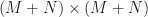
These spikes in the solutions to the design equations are fairly common, although I was able to avoid them in the various examples I provided up to this point. I also track the condition number of the matrix $\mathbf{S}$ as the design equations are being solved. For the present case, a zoomed-in version of the plot of the condition number (versus frequency $f$ ) and the total energy in the matrix $\mathbf{S}$ is shown in Figure 25.

Figure 25. A portion of the plot of condition number of $\mathbf{S}$ versus frequency for the FRESH filter using the shifts in (53) and also using 32768 samples to approximate the spectral correlation functions used in the design equations. Note the large increase in the condition number at the locations of the two spikes in the transfer functions of Figure 24.

So the matrix $\mathbf{S}$ is close to being singular at/near these two frequencies. Why? Is this an inherent property of the spectral correlation functions and the design equations for this particular example? Is it due to poor estimates?

If we increase the number of samples used to estimate the spectral correlation functions needed to solve the design equations to 131072, we eliminate the spikes and the resulting output NMSE is a much more reassuring -11.0 dB. The transfer functions are shown in Figure 26.

Figure 26. FRESH-filter branch transfer functions for the motivating problem and the frequency shifts given by (53). Here the design equations are solved using estimates of the spectral correlation function obtained using 131072 samples of data. Note the absence of the large spikes in the transfer functions on either side of $f=0$ that are evident in Figure 24.

Figure 26. FRESH-filter branch transfer functions for the motivating problem and the frequency shifts given by (53). Here the design equations are solved using estimates of the spectral correlation function obtained using 131072 samples of data. Note the absence of the large spikes in the transfer functions on either side of $f=0$ that are evident in Figure 24.

The spikes in the transfer functions cause the error spectrum to be much more energetic, which is consistent with the large NMSEs we see whenever we use such transfer functions in the FRESH filter. The error spectrum for the short-input case of Figure 24 is shown in Figure 27 and for the long-input case of Figure 26 in Figure 28.

Figure 27. Error spectrum corresponding to the short-input case of Figure 24. Here the design equations are solved by using spectral correlation estimates obtained from a data vector having 32768 samples. Note the large energy in the error for frequencies near the spikes.

Figure 28. Error spectrum corresponding to the long-input case of Figure 26. Here the design equations are solved by using spectral correlation estimates obtained from a data vector having 131072 samples. Note the small energy in the error for all frequencies.

The problem is that we would very much like to solve the design equations using a small number of samples, as this might render FRESH filtering more practical. One possible approach is to track the derivative of the condition number and when it exceeds a threshold, instead of accepting the solution to the design equations, perform interpolation using nearby transfer-function values that correspond to smaller condition numbers.

I’ve talked with other researchers that have encountered the spikes in the design-equation-obtained transfer functions, and they have employed completely independent software to implement their system, so I’m confident that this isn’t a peculiar fluke of my own set of software tools.

Concluding Remarks and Research Questions

We see that FRESH filtering is a complicated idea and a complex set of signal-processing software tools are needed to implement it. We have skipped over describing possible practical adaptation methods–perhaps that will appear in a future CSP Blog post. There are many other signal types and signal combinations to study as well.

Here are some questions that I think would be valuable to investigate as a signal-processing researcher.

For a given signal and interference scenario, how do we pick good frequency shifts? We’d like an algorithm that can find a minimal set of shifts that provides output NMSE to within $X$ dB of the cyclic Wiener filter for the scenario.
What is the best way to solve the design equations using data? Here we’ve used the FSM with a smoothing window width of 2 percent of the sampling rate. Might more sophisticated methods or more complex smoothing windows help reduce the prevalence of the spikes when forming estimates with relatively short input-data blocks?
What are the fundamental reasons for the occurrence of the transfer-function spikes? Some choices of frequency shifts present no spikes–the condition number of $\mathbf{S}$ is low and constant across the entire signal band. Others provide multiple spikes.
Can the transfer-function spikes always be removed or attenuated by simply increasing the time-bandwidth product (resolution product) of the spectral correlation estimates used in the design equations? Are there situations where $\mathbf{S}$ is singular simply due to the nature of the signal-separation problem and its parameters?
In almost all cases I’ve run, the adaptive FRESH filter produces smaller NMSE than the corresponding design-equation-solution FRESH filter. Is this always due to the imperfect solution of the design equations implied by the use of spectral correlation estimates instead of theoretical spectral correlation function values?

If you’ve found significant value in this post, please consider donating to the CSP Blog to keep it ad-free and keep the posts and datasets coming.

Author: Chad Spooner

I'm a signal processing researcher specializing in cyclostationary signal processing (CSP) for communication signals. I hope to use this blog to help others with their cyclo-projects and to learn more about how CSP is being used and extended worldwide. View all posts by Chad Spooner

10 thoughts on “Frequency Shift (FRESH) Filtering for Single-Sensor Cochannel Signal Separation”

chaoqi says:

March 3, 2023 at 7:57 pm

I have been looking forward to the post about the FRESH filter for a long time, and I will find time to read it carefully. Thank you for your sharing. I have seen the video you explained before.

Loading...

Reply
1. Chad Spooner says:
  
  March 4, 2023 at 7:59 am
  
  Welcome to the CSP Blog Comments chaoqi! Sorry I took so long getting that post out. I think I’m now in a good position to render some “Comments On …” FRESH-filtering papers that have been accumulating in my files. Enjoy, and please let me know your thoughts on the strengths and weaknesses of the post, and most especially errors in the post.
  
  Loading...
  
  Reply
SADOK_MU says:

March 27, 2023 at 11:29 pm

Thank you professor for your efforts…after reading every article, I get more insights on the subject of cyclo-stationarity.

After my first reading, I don’t catch why the eq 11 and 12 take these form? Did you imposed the form of the time varying impulse response? The eq 12 I didn’t understand because a little differences with classical Fourier coefficients…

Can the concept of “non-circular” (Dr. Picinbono) or equivalently “improper” (Dr. Shereier) signal explain also the necessity to use an additional complex conjugate input to the FRESH filter?

Loading...

Reply
1. Chad Spooner says:
  
  March 28, 2023 at 3:03 pm
  
  I don’t catch why the eq 11 and 12 take these form?
  
  I am progressing through several possible forms for the signal processor that is to perform signal separation: linear time-invariant, general time-variant, periodically time-variant, and almost periodically time-variant. Each time, yes, the form is imposed on the processor.
  
  Did you imposed the form of the time varying impulse response?
  
  Yes. The question “What is the best signal separator if the separator is constrained to be a linear time-invariant system?” is answered by “The Wiener filter if the figure of merit is mean-squared error.” Now we ask the question “What is the best signal separator if the separator is constrained to be a linear periodically (or almost periodically) time-variant system?” And the answer is “The cyclic Wiener filter.”
  
  eq 12 I didn’t understand because a little differences with classical Fourier coefficients…
  
  The Fourier-series formula in (12) uses an infinite time average instead of the usual Fourier-series average over a single period. This is to simultaneously accommodate both periodic systems and almost periodic systems. See The Literature [R8] and [R131].
  
  Can the concept of “non-circular” (Dr. Picinbono) or equivalently “improper” (Dr. Shereier) signal explain also the necessity to use an additional complex conjugate input to the FRESH filter?
  
  Yes. Those two researchers were a bit late to the party, though. I still recall, with some amusement, Schreier and Scharf at Asilomar 2001 explaining about random variables with non-zero second-order moments where one does not conjugate one of the factors (“improper”)! They were surprised and amazed and expected the listeners in the audience to be so too. I raised my hand and said “I’m not surprised or amazed. We’ve been using so-called “improper” variables for years and publishing about it too. They arise naturally in mathematical models of communication signals.” But those researchers you cite are from the statistics school of electrical engineering. They don’t pay attention to the signal-processing school. Their training has, unfortunately, led them to focus on Gaussian random variables and strict proofs of estimator consistency. They end up being late to the application side of things, especially in communication signal processing.
  
  Loading...
  
  Reply
  1. SADOK_MU says:
    
    March 29, 2023 at 1:04 am
    
    Thank you professor for your answers.
    
    I agree with you about statistic school but I think sometimes it brings more insights about the subject.
    
    Do you have any recommended works about processing non-gaussian signals and interferences ? Volterra structure, in addition to its complexity in most cases it modifies noise distribution and make hard subsequent processing like detection or estimation.
    
    It’s a great pleasure to have such an opportunity to exchange with you, professor.
    
    Best regards.
    
    Loading...
    
    Reply
    1. Chad Spooner says:
      
      March 29, 2023 at 2:01 pm
      
      Do you have any recommended works about processing non-gaussian signals and interferences ?
      
      Almost every signal that I process using CSP is non-Gaussian. The noise associated with receiving a non-Gaussian communication signal using a physical radio receiver is Gaussian. But all the signals in the Gallery are non-Gaussian, except analog AM because I typically generate the message signal there as a bandlimited Gaussian signal.
      
      Academic papers and books sometimes focus on Gaussian cyclostationary signals, but such signals don’t come up for me in real-world work.
      
      Does that answer your question?
      
      Loading...
      
      Reply
      1. SADOK_MU says:
        
        March 29, 2023 at 2:16 pm
        
        I meant is there any nonlinear structure other than volterra one to deal with non-gaussian signals ? From statistical perspective, optimal solution isn’t linear one but nonlinear in non Gaussian scenario.
        
        Optimal nonlinear structure modifies background noise (e.g. PDF) which create other challenges to subsequent processing…What is your opinion on this issue ?
        
        Recently, I heard about Signal Processing in generalized metric space with new nonlinear operation. Do you have any feedback on this question ?
        
        Loading...
Jason Williams says:

February 7, 2024 at 3:19 pm

Thank you Chad for this post! It was an invaluable companion piece to “Cyclic Wiener filtering: theory and method” to better my understanding of FRESH/Cyclic Wiener filtering concepts, especially the walkthrough of your motivating example. Might I suggest a subtitle (punny, although funny may be a stretch)? “Getting mixed signals? Keep it FRESH!”

Loading...

Reply
George Zlovik says:

March 20, 2024 at 12:55 am

Hi, many thanks for your blog. I have just recently became aware of it, and I already find it useful.
I have some questions following your post:
1. When using the Weiner filter you write – “We use the FSM to estimate the power spectra needed to form the filter’s transfer function in (5). ”
When using the FRESH filter you write – “We choose to solve the design equations using spectral correlation estimates in place of the theoretical spectral correlation functions and these estimates are formed using the frequency-smoothing method applied to 32,768 samples of the observable data and the reference signal d(t). ”
So is there some assumption being made about knowing the desired/reference signal apriori?
What happens if we don’t know the reference signal apriori, but rather only have some coarse knowledge of what its CF might be?
2. You assume different carrier offsets and bit rates for the signals, which in turn implies different CFs for them. What would happen if some of the parameters would have been the same? Say, same bit rate but different carrier offsets, would it still be possible to filter out the interferences?

Loading...

Reply
1. Chad Spooner says:
  
  March 20, 2024 at 9:25 am
  
  Welcome to the CSP Blog George! Thanks much for the thoughtful comment.
  
  So is there some assumption being made about knowing the desired/reference signal apriori?
  
  When solving the design equations (39), you need the spectral correlation functions for the data as well as the cross spectral correlation functions between the desired signal and the data (right-hand side). The latter includes the power spectrum for the desired signal. If you know that in advance, you can just use it. If you have a good model for the desired signal, you can do as I say. For all the other spectral correlation functions, you can, in principle, estimate them from the received data, or you can use analytical formulas, depending on the problem set up. The thing that is hard to estimate directly from the data is the power spectrum of the desired signal, because signal-selectivity doesn’t apply.
  
  What happens if we don’t know the reference signal apriori, but rather only have some coarse knowledge of what its CF might be?
  
  I address the issue of estimating the required cycle frequencies, blindly, from the data itself in the post section called “Estimating Interferer Cycle Frequencies and Cycle-Frequency Patterns Blindly from Received Data.”
  
  What would happen if some of the parameters would have been the same? Say, same bit rate but different carrier offsets, would it still be possible to filter out the interferences?
  
  If the symbol rates were identical, but the carrier offsets were different, and the signal type is BPSK or MSK (some signal with conjugate cyclostationarity), I think performance would be similar to the examples I’ve shown. If all of the cycle frequencies are shared by the two signals, then they completely spectrally overlap, and the problem is more difficult. In principle, FRESH filtering could still provide some separation, provided that the symbol-clock and carrier phases weren’t also identical. To see how the FRESH approach might work, you could evaluate the error spectrum (45) for this kind of problem.
  
  Loading...
  
  Reply