SPTK: The Laplace Transform – Cyclostationary Signal Processing

Previous SPTK Post: MATLAB’s resample.m Next SPTK Post: Practical Filters

In this Signal Processing ToolKit post, we look at a generalization of the Fourier transform called the Laplace Transform. This is a stepping stone on the way to the Z Transform, which is widely used in discrete-time signal processing, especially in control theory.

Jump straight to ‘Significance of the Laplace Transform in CSP‘ below.

Let’s motivate the upcoming Z transform by generalizing the Fourier transform. But why do we need to generalize something so pure, so good, so useful, and so perfect as the Fourier transform???

Consider the unit-ramp function $r(t)$ shown in Figure 1. Recalling that the unit-step function $u(t)$ is zero for negative $t$ , one for positive $t$ , and variously defined as one or zero for $t=0$ (let’s not worry about that), the unit-ramp can be expressed as $r(t) = tu(t)$ .

Figure 1. The unit-ramp function $r(t) = tu(t)$ .

Figure 1. The unit-ramp function $r(t) = tu(t)$ .

What is the Fourier transform of $r(t)$ ? We can start by writing it down,

$\displaystyle R(f) = {\cal{F}}\left[ r(t) \right] \hfill (1)$

$\displaystyle = \int_{-\infty}^\infty tu(t) e^{-i 2 \pi f t} \, dt. \hfill (2)$

An expression for this Fourier transform can be found, but it involves the derivative of the impulse function, so it doesn’t exist as a well-behaved function, and is even difficult to deal with as a generalized function.

Consider also random functions like Gaussian noise and exponentials like $e^{at}u(t)$ with $a > 0$ . They do not have Fourier transforms. For the exponentials and ramps, the basic problem is that the functions are increasing with $t$ (or whatever the independent variable is) and so the integral–which is the limit of a sum involving the values of that increasing function–cannot converge. For sample paths of random processes like the Gaussian process or a BPSK signal, the limit simply does not converge to any particular value, although the signal does not blow up like the ramp and exponentials.

One way around this lack of convergence in the Fourier transform is to introduce a damping factor inside the transform’s integral to ensure that the signal does not increase with time so much that the integral diverges. For example, if we multiply the unit ramp by a unit exponential $e^{-t}$ and integrate the result, we get a finite number. This exponential dampening is illustrated in Figure 2.

Figure 2. Illustration of the power of a decaying exponential factor to render an unintegrable function like $r(t) = tu(t)$ integrable.

The exponential $e^{-at}$ tends to zero rapidly, and controllably with the magnitude of the positive number $a$ , and is never zero, so it is a good choice to both preserve the character of the signal it is multiplying (since it is never zero, no values of that function are discarded in the integration) and to ensure that no matter how fast the function under study increases with time, it can be brought down to earth.

So to enable a transform of a signal that is not Fourier transformable, we enter a factor of $e^{-\sigma t}$ , for some real number $\sigma$ , into our Fourier transform as follows

$\displaystyle \int_{-\infty}^\infty \underbrace{x(t)}_{Signal} \underbrace{e^{-\sigma t}}_{\substack{Damping\\ Factor}} \underbrace{e^{-i2\pi f t}\, dt.}_{\substack{Sine\ Wave\\ with\ Frequency\ f\\ and \ Amplitude\ dt}} \hfill (3)$

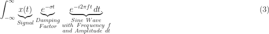
Now let the variable $s$ be equal to $\sigma + i2\pi f$ . Then our transform becomes

$\displaystyle X(s) = \int_{-\infty}^\infty x(t) e^{-st} \, dt, \hfill (4)$

which is the Laplace transform of $x(t)$ . Most of the time we want to apply this transform to signals $x(t)$ that are zero for negative times $t$ , so that the Laplace transform is one-sided and is usually written as

$\displaystyle X(s) = \int_0^\infty x(t) e^{-st} \, dt, \hfill (5)$

but the two-sided transform is also used. The one-sided transform, being applicable to signals that are zero for negative time, is particularly useful for transformation of causal impulse-response functions, which possess that exact property already.

The advantage of the Laplace transform over the Fourier transform is that the functions to be transformed can be poorly behaved–they might correspond to systems that are unstable and so their outputs grow without bound. So you might be able to see why we’ve done without the Laplace transform at the CSP Blog lo these many years–we are almost always interested in communication signals that are perhaps not Fourier transformable but are not growing without bound. We got around the fact that random communication signals (that is, all useful communication signals) are not Fourier transformable by switching our focus from transforms to power spectra.

If the Fourier transform $X(f)$ for $x(t)$ exists, then it is given by the Laplace transform $X(s)$ with $\sigma = 0 \Rightarrow s = i2\pi f$ . Following our notation convention for the Fourier transform, the Laplace transform is denoted by the operator ${\cal{L}} [\cdot]$ and also the doubled-ended arrow $\Longleftrightarrow$ as in

$\displaystyle X(s) = {\cal{L}}\left[ x(t) \right] = \int_0^\infty x(t) e^{-st} \, dt \hfill X(s) \Longleftrightarrow x(t). \hfill (6)$

Linearity

Since the transform is defined by an integral, and integration is itself linear, it follows that the Laplace transform, like the Fourier transform, is a linear transform. This simply means that the Laplace transform of the sum of scaled signals is the sum of scaled Laplace transforms,

$\displaystyle {\cal{L}} \left[a_1 x_1(t) + a_2 x_2(t) \right] = a_1 {\cal{L}} \left[x_1(t)\right] + a_2 {\cal{L}} \left[x_2(t)\right] = a_1X_1(s) + a_2 X_2(s). \hfill (7)$

Linearity will help us compute the Laplace transform of complicated signals by permitting us to express them as the sum of simpler signals, find the Laplace transform of each of the summands, and finally add them up.

Region of Convergence in the s-Plane

For what values of $\sigma$ does a particular Laplace transform exist? This is typically visually expressed by considering the $s$ -plane, which has vertical axis denoted by $\omega$ , which equals $2\pi f$ , or by $f$ itself, and horizontal axis denoted by $\sigma$ . Let’s take a look at the region of convergence by taking our first Laplace transform: the transform of the exponential function $f(t) = e^{-at}u(t)$ .

Let’s go through the math. Applying the definition of the transform,

$\displaystyle {\cal{L}}\left[ f(t) \right] = F(s) = \int_0^\infty e^{-at} u(t) e^{-st}\, dt \hfill (8)$

$\displaystyle = \int_0^\infty e^{-(a+s)t} \, dt. \hfill (9)$

Formally, this integral equals

$\displaystyle F(s) = \left. \frac{1}{-(a+s)} e^{-(a+s)t} \right|_{t=0}^\infty \hfill (10)$

$\displaystyle = \left. \frac{1}{-(a + \sigma + i2\pi f)} e^{-(a + \sigma + i2\pi f)} \right|_{t=0}^\infty . \hfill (11)$

If $(a + \sigma) > 0$ , then $\displaystyle \lim_{t\rightarrow\infty} e^{-(a+\sigma + i2\pi f)} \rightarrow 0$ , and also we won’t divide by zero because $\left| a+\sigma + i2\pi f \right| \neq 0$ for any $f$ . With the condition $a + \sigma > 0$ , then, the transform is

$\displaystyle F(s) = \frac{1}{a + s}, \ \ \ \sigma > -a. \hfill (12)$

The convergence parameter $\sigma$ in $s$ must be greater than $-a$ for the integral to exist, which can be satisfied whether or not $a$ is positive or negative (whether or not the exponential decreases or increases as time $t$ increases).

When $a> 0$ , the exponential is decreasing, and the region of convergence looks like the shaded area in Figure 3. Since $a$ is positive, $-a$ is negative, and the region of convergence includes a part of the $s$ -plane where $\sigma <0$ and all of the half plane for $\sigma \ge 0$ . In particular, the region of convergence contains the $f$ axis, where $\sigma = 0$ . This means that the Laplace transform formula is valid if we substitute $\sigma = 0$ into (12), which is the Fourier transform of $e^{-at}u(t)$ ,

$\displaystyle F(f) = F(s|\sigma=0) = \frac{1}{a + i2\pi f}, \hfill (13)$

which indeed matches the Fourier transform for the decaying exponential obtained by direct computation of the Fourier transform.

The important point is that if the Laplace transform formula corresponds to a region of convergence that includes the $f$ axis, the Fourier transform can easily be determined from the Laplace transform. If the region of convergence does not contain the $f$ axis, then the Fourier transform cannot be determined from the Laplace transform. The Fourier transform in such cases does not exist in the normal sense of a function, but may exist if generalized functions such as impulses are permitted. We’ll see examples shortly.

Figure 3. Illustration of the region of convergence for the Laplace transform integral when the function to be transformed is the exponential $e^{-at}u(t)$ with positive $a$ . Note that the region of convergence contains the $f$ axis, which implies that the Fourier transform of the function exists and can be computed by setting $\sigma = 0$ in $F(s) = F(\sigma + i 2 \pi f)$ .

Figure 3. Illustration of the region of convergence for the Laplace transform integral when the function to be transformed is the exponential $e^{-at}u(t)$ with positive $a$ . Note that the region of convergence contains the $f$ axis, which implies that the Fourier transform of the function exists and can be computed by setting $\sigma = 0$ in $F(s) = F(\sigma + i 2 \pi f)$ .

If $a < 0$ , then the region of convergence is wholly contained in the right-half plane as illustrated in Figure 4. The $f$ axis is not contained in this region, so that the Fourier transform of the increasing exponential does not exist.

What about when $a=0$ ? The function under consideration is $f(t) = e^{-at}u(t) = e^{o}u(t) = u(t)$ , or just the unit-step function itself. The condition on $\sigma$ remains, which is $\sigma > -a \Rightarrow \sigma > 0$ , and under this condition

$\displaystyle u(t) \Longleftrightarrow \frac{1}{a+s} = \frac{1}{s} \hfill \sigma > 0. \hfill (14)$

You might recall that the Fourier transform of the unit-step function is not a particularly friendly function,

$\displaystyle {\cal{F}}[u(t)] = U(f) = \frac{1}{2}\delta(f) + \frac{1}{i2\pi f}, \hfill (15)$

which invites the question of what is going on in $U(f)$ at $f= 0$ . Compare that expression to the Laplace transform expression of $1/s$ with $\sigma >0$ . Better! Not your best friend (that is rectangular-pulse BPSK of course), to be sure, but friendly enough.

At this point in the development, we have the Laplace transforms of the unit-step function and the exponential function. We’d like to know a lot more if we want to try to apply the transform to problems involving signals and systems. To do that, we could apply the Laplace integral (5) to each of a number of signals we’ve encountered in the SPTK posts, but it is typically easier to try to be more clever. We’d like to understand how common mathematical operations, such as scaling, differentiation, integration, convolution, multiplication, etc., affect a signal’s transform. Then when we encounter a new signal, we try to express that signal in terms of one or more of these operations on a signal for which we already know the transform.

Mathematical Operations

Scaling by a Constant

What is the Laplace transform of the signal $af(t)$ , for any complex constant $a$ , given that we know $F(s) \Longleftrightarrow f(t)$ ? Since we already know that the Laplace transform is linear, it follows easily that the transform of the scaled signal is the scaled transform,

$\displaystyle af(t) \Longleftrightarrow aF(s). \hfill (16)$

Differentiation

Suppose we have a differentiable function $f(t)$ ,

$\displaystyle f^\prime(t) = \frac{d}{dt} f(t), \hfill (17)$

with Laplace transform $F(s)$ . What is ${\cal{L}}[f^\prime(t)]$ ? The transform integral (5) is

$\displaystyle {\cal{L}} \left[ f^\prime (t) \right] = \int_0^\infty f^\prime (t) e^{-st} \, dt. \hfill (18)$

We can proceed to evaluate this kind of integral by applying the technique called integration by parts.

\displaystyle \left. \int_a^b u(x) v^\prime (x) \, dx = u(x)v(x)\right|_{x=a}^b - \int_a^b u^\prime (x) v(x) \, dx

\displaystyle v^\prime (x) = \frac{d}{dx} v(x)

The first step is crucial: Identify $u(t)$ and $v^\prime (t)$ from the integrand components of the integral to be solved. We’ll make the choice $u(t) = e^{-st}$ and $v^\prime(t) = f^\prime (t)$ ,

$\displaystyle {\cal{L}}\left[ f^\prime (t) \right] = \int_0^\infty \underbrace{\left( e^{-st} \right)}_u \underbrace{\left( f^\prime (t) \right)}_{v^\prime} \, dt. \hfill (19)$

With this choice for $u$ and $v^\prime$ , we can identify $u^\prime$ and $v$ ,

$\displaystyle v(t) = f(t) \hfill (20)$

$\displaystyle u^\prime (t) = -se^{-st}. \hfill (21)$

With this choice, let’s carefully follow the integration-by-parts rule.

$\displaystyle \left. {\cal{L}}\left[ f^\prime (t) \right] = e^{-st}f(t) \right|_{t=0}^\infty - \int_0^\infty (-se^{-st})f(t) \, dt. \hfill (22)$

If $\sigma > 0$ , then $e^{-st} = e^{-\sigma t}e^{-i2\pi f t} \rightarrow 0$ as $t \rightarrow \infty$ , so that

$\displaystyle {\cal{L}} \left[ f^\prime (t) \right] = 0 - e^{-s(0)} f(0) + s\int_0^\infty f(t) e^{-st} \, dt \hfill (23)$

$\displaystyle = sF(s) - f(0). \hfill (24)$

We adopt the convention of my beloved The Literature [R132], and interpret $f(0)$ to be $f(0^-)$ , the value of the function just before zero, to get around certain technical issues involving discontinuities at $t=0$ , such as might occur for certain causal linear time-invariant systems‘ impulse-response functions. So the final answer for the derivative of $f(t)$ is

$\displaystyle f^\prime (t) \Longleftrightarrow sF(s) - f(0^-). \hfill (25A)$ .

As a preview, since we know that $U(s) = 1/s \Longleftrightarrow u(t)$ , and $u^\prime (t) = \delta(t),$ then $\Delta(s) = 1 \Longleftrightarrow \delta(t)$ , which is consistent with ${\cal{F}}\left[ \delta(t) \right] = 1$ , as we’ve seen before.

It follows immediately that the Laplace transform of the second derivative of $f(t)$ ( $f^{\prime\prime} (t)$ ) is

$\displaystyle f^{\prime\prime}(t) \Longleftrightarrow s^2F(s) - sf(0^-) - f^\prime(0^-). \hfill (25B)$

Integration

Next let’s look at differentiation’s inverse operation: integration. What is the Laplace transform of $\displaystyle \int_0^t f(\tau) \, d\tau$ ?

$\displaystyle {\cal{L}} \left[ \int_0^t f(\tau)\, d\tau \right] = {\cal{L}} \left[ g(t) \right] = \int_0^\infty g(t) e^{-st} \, dt. \hfill (26)$

Let’s again reach for integration by parts. Since the integral of $e^{-st}$ is easy, let’s choose that for $v^\prime$ ,

$\displaystyle u^\prime (t) = \frac{d}{dt} g(t) = \frac{d}{dt} \int_0^t f(\tau) \, d\tau = f(t) \hfill (27)$

$\displaystyle v(t) = \int v^\prime (t) \, dt = \frac{1}{-s} e^{-st}. \hfill (28)$

Our formula reduces to

$\displaystyle {\cal{L}} \left[ g(t) \right] = \left. {\cal{L}} \left[ \int_0^t f(\tau)\, d\tau \right]= g(t)\left(\frac{-1}{s}\right)e^{-st}\right|_{t=0}^\infty - \int_0^\infty f(t) \left(\frac{-1}{s} e^{-st}\right) \, dt. \hfill (29)$

If $\sigma > 0$ , $\displaystyle \lim_{t\rightarrow\infty} g(t)$ is finite, and $g(0) = 0$ no impulse in $f(t)$ at the origin), then the first term on the right in (29) is zero. We are left with

$\displaystyle {\cal{L}} \left[ g(t) \right] = \frac{1}{s} \int_0^\infty f(t) e^{-st} \, dt = \frac{1}{s} F(s), \hfill (30)$

which is satisfying because the effect of differentiation (factor of $s$ ) undoes the effect of integration (factor of $1/s$ ). The final result is

$\displaystyle \int_0^t f(\tau)\, d\tau \Longleftrightarrow \frac{1}{s} F(s), \hfill \sigma > 0. \hfill (31)$

As a preview, consider that the unit ramp $r(t) = tu(t)$ is the integral of the unit step

$\displaystyle r(t) = tu(t) = \int_0^t u(\tau) \, d\tau. \hfill (31)$

What does that imply about $R(s)$ ?

Time Scaling

Suppose $F(s) \Longleftrightarrow f(t)$ . What is ${\cal{L}}\left[ f(at) \right]$ ?

First, let’s rule out $a=0$ because then we don’t have a function of time anymore–we’d be asking about the Laplace transform of $f(0)$ , which is the Laplace transform of a constant, which we already know is $f(0)/s$ . But let’s also rule out $a < 0$ , because those values of $a$ not only compress or expand the time axis, but they swap all the function values for negative time with those for positive time. Yet $F(s)$ is itself only on function of $f(t)$ for $t \ge 0$ . So we wouldn’t be able to say anything about the relationship between ${\cal{L}}\left[ f(t) \right]$ and ${\cal{L}} \left[ f(at) \right]$ if $a < 0$ . That leaves the still-considerable set of $a$ that are real numbers greater than zero.

Let’s proceed by evaluating the Laplace integral (5).

$\displaystyle {\cal{L}}\left[f(at)\right] = \int_0^\infty f(at) e^{-st}\, dt. \hfill (32)$

Let’s do a substitution for the variable of integration:

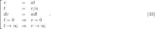
$\displaystyle \left[ \begin{array}{lll} v & = & at \\ t & = & v/a \\ dv & = & a dt \\ t=0 & \Rightarrow & v= 0 \\ t\rightarrow\infty & \Rightarrow & v \rightarrow \infty \end{array} \right. . \hfill (33)$

This substitution leads to

$\displaystyle {\cal{L}} \left[ f(at) \right] = \int_0^\infty f(v) e^{-sv/a} (1/a) \, dv \hfill (34)$

$\displaystyle = \frac{1}{a} \int_0^\infty f(v) e^{-(s/a)v} \, dv \hfill (35)$

$\displaystyle = \frac{1}{a} F(s/a). \hfill (36)$

The final result is, in our compact notation,

$\displaystyle f(at) \Longleftrightarrow \frac{1}{a} F(s/a). \hfill (37)$

Multiplication by t

We are interested here in $\displaystyle {\cal{L}} \left[ tf(t) \right]$ , but let’s guess at the answer first and then work backward to verify. We know that $sF(s)$ is the transform of the derivative of $f(t)$ , so if there is any significant duality between time $t$ and complex frequency $s$ in the Laplace transform, we might guess that the transform of $tf(t)$ is the derivative of $F(s)$ . And since the Laplace transform and Fourier transform are closely related, and the Fourier transform does possess duality, we have good reason to make this guess. Let’s check.

$\displaystyle \frac{d}{ds} F(s) = \frac{d}{ds} \int_0^\infty f(t) e^{-st} \, dt \hfill (38)$

$\displaystyle = \int_0^\infty f(t) \left( \frac{d}{ds} e^{-st}\right) \, dt \hfill (39)$

$\displaystyle = \int_0^\infty f(t) (-t) e^{-st} \, dt \hfill (40)$

$\displaystyle = - \int_0^\infty (tf(t)) e^{-st} \, dt, \hfill (41)$

$\displaystyle tf(t) \Longleftrightarrow - \frac{d}{ds} F(s). \hfill (42)$

Apart from the negative sign, the guess is verified.

Delay (Time Shift)

A delayed version of $f(t)$ is $f(t-t_0)$ with $t_0 \ge 0$ . This delay pushes the signal forward in time (to the right along the time axis). What is the Laplace transform of the delayed signal in terms of the known transform of the original signal $F(s)$ ? (You might guess based on the behavior of the Fourier series and transform for delayed signals.)

We have to be a little careful about delaying $f(t)$ here because it may be nonzero for negative time, and when $t_0 > 0$ , some of the function defined for negative time shifts into positive time, yet none of that portion of $f(t)$ was used to find $F(s)$ .

So what we want to consider is $f(t)u(t)$ , ensuring that the function is zero for all negative time, and its delayed version $f(t-t_0)u(t-t_0)$ . Otherwise, if we want to deal with the negative-time portion of $f(t)$ , we can use the two-sided Laplace transform.

We’ll proceed directly to the definition (5),

$\displaystyle {\cal{L}}\left[ f(t-t_0)u(t-t_0)\right] = \int_0^\infty f(t-t_0)u(t-t_0)e^{-st} \, dt. \hfill (43)$

We require a change of variables,

$\displaystyle \left[ \begin{array}{lll} v & = & t-t_0 \\ t & = & v+t_0 \\ dv & = & dt \\ t=0 & \Rightarrow & v= -t_0 \\ t\rightarrow\infty & \Rightarrow & v \rightarrow \infty \end{array} \right. . \hfill (44)$

Applying this change of variables leads to

$\displaystyle {\cal{L}}\left[f(t-t_0)u(t-t_0)\right] = \int_{-t_0}^\infty f(v)u(v)e^{-s(v+t_o)} \, dv. \hfill (45)$

Since $t_0 > 0$ , and the integrand is zero for $v \in [-t_0, 0^-]$ , we have

$\displaystyle {\cal{L}}\left[f(t-t_0)u(t-t_0)\right] = \int_0^\infty f(v)u(v)e^{-sv}\,dv e^{-st_0}, \hfill (46)$

$\displaystyle f(t-t_0)u(t-t_0) \Longleftrightarrow F(s)e^{-st_0}, \hfill t_0 \ge 0. \hfill (47)$

Delay (s Shift)

If we shift a Laplace transform by some amount $a$ , as in $F(s+a)$ , what is the corresponding time function? If we had an easy-to-evaluate inverse transform, we could apply it here. But we’ve avoiding introducing the inverse Laplace transform so far (for good reason), so let’s once again take a guess, and see if that leads to easy analysis.

We know that a shift in frequency for the Fourier transform is a multiplication of the time waveform by a complex exponential,

$\displaystyle F(f-f_0) \Longleftrightarrow f(t)e^{i2\pi f_o t}, \hfill (48)$

so we can guess that multiplication of the time waveform by something like $e^{at}$ will produce a shifted version of the Laplace transform. Let’s work it out.

$\displaystyle {\cal{L}}\left[e^{at}f(t)u(t)\right] = \int_0^\infty f(t) e^{-(s-a)t} \, dt \hfill (49)$

$\displaystyle = F(s-a), \hfill (50)$

which implies the desired result

$\displaystyle e^{-at}f(t)u(t) \Longleftrightarrow F(s+a). \hfill (51)$

Convolution

Suppose we have two causal signals $f(t)u(t)$ and $g(t)u(t)$ . Then their (normal) convolution is also causal in that

$\displaystyle [f(t)u(t)] \otimes [g(t)u(t)] = h(t) = h(t)u(t). \hfill (52)$

So all three signals are of the usual sort we are dealing with as we study the one-sided Laplace transform.

What is $H(s) = {\cal{L}}\left[h(t)u(t)\right]$ ? Again, we can make a very good guess by reflecting on the convolution theorem: $F(s)G(s)$ . I’ll leave the proof as an exercise for the interested reader.

Periodic Signals

Let’s look at the case of a generic periodic signal. Let the period of the signal be $T > 0$ . Then the defining characteristic of the periodic signal $f(t)$ is that $f(t+T) = f(t)$ for all real numbers $t$ .

Periodic signals can be written in a lot of equivalent ways because all that is required is that the function over some interval $[t_1, t_1+T)$ is replicated at every other interval $[t_1+kT, t_1+(k+t)T)$ . Consider the periodic rectangular pulse train shown in Figure 5.

Figure 5. A periodic rectangular-pulse pulse train ( $T > U$ ).

Figure 5. A periodic rectangular-pulse pulse train ( $T > U$ ).

Recalling that the function $\mbox{\rm rect} (t)$ is defined as being equal to one on $[-1/2, 1/2]$ and zero otherwise, it is natural to express $f(t)$ in Figure 5 as

$\displaystyle f(t) = \sum_{k=-\infty}^\infty A\,\mbox{\rm rect} \left( (t-kT)/U \right). \hfill (53)$

But for the Laplace transform we’re considering here, we only care about the function for non-negative times $t$ . We can express the signal in a Laplace-transform friendly way by using the Base Period shown in Figure 5,

$\displaystyle p_0(t) = A\, \mbox{\rm rect} (2(t-U/4)/U) + A\, \mbox{\rm rect} (2(t-(T-U/4))/U). \hfill (54)$

Then the entire signal can be expressed as

$\displaystyle f(t) = \sum_{k=-\infty}^\infty p_0(t - kT ), \hfill (55)$

and therefore the positive-time portion of $f(t)$ is easily expressed as the truncated sum

$\displaystyle f(t) = \sum_{k=0}^\infty p_0(t - kT), \ \ \ t \ge 0. \hfill (56)$

To find $F(s) = {\cal{L}}\left[f(t)\right]$ here, we can invoke the established linearity and time-delay properties of the transform to yield

$\displaystyle F(s) = \sum_{k=0}^\infty P_0(s)e^{-skT}, \hfill (57)$

where $P_0(s) \Longleftrightarrow p_0(t)$ .

Some Laplace Transforms

Now let’s derive some Laplace transforms for some simple signals that we frequently encounter in signal analysis, such as the unit-step function $u(t)$ , the ramp function $r(t) = tu(t)$ , the trigonometric functions, exponentials with real exponents, exponentials with imaginary exponents (sine waves), the rectangular pulse train, etc.

The Impulse Function (Delta Function)

Let’s start with $f(t) = \delta(t)$ , where $\delta(t)$ is the impulse function or Dirac’s delta function. Applying the Laplace transform definition directly gives the answer in short order, due to the sifting property of the impulse function and the fact that it integrates to unity,

$\displaystyle F(s) = \int_0^\infty \delta(t) e^{-st} \, dt = \int_0^\infty \delta(t) e^0 \, dt = 1 \hfill (58)$

$\displaystyle \delta(t) \Longleftrightarrow 1. \hfill (59)$

The Unit-Step Function

The unit-step function $u(t)$ is zero for all negative time and one for positive time and is variously defined at $t=0$ ,

$\displaystyle u(t) = \left\{ \begin{array}{ll} 0, & t < 0 \\ 1, & t \ge 0 \end{array} \right. . \hfill (60)$

For $f(t) = u(t)$ , we have

$\displaystyle F(s) = U(s) = \int_0^\infty u(t) e^{-st} \, dt = \int_0^\infty e^{-st}\, dt \hfill (61)$

$\displaystyle = \left. \frac{e^{-st}}{-s} \right|_{t=0}^\infty. \hfill (62)$

Now, if $\sigma > 0$ , then $e^{-st} = e^{-\sigma t - i2\pi f t} \rightarrow 0$ as $t \rightarrow \infty,$ so that

$\displaystyle U(s) = 0 - \left(\frac{1}{-s}\right) = \frac{1}{s} \hfill (63)$

$\displaystyle u(t) \Longleftrightarrow \frac{1}{s}. \hfill (64)$

Alternatively, we can observe that the unit-step function is the integral of the impulse function

$\displaystyle u(t) = \int_{-\infty}^\infty \delta(t) \, dt$

and apply the integration formula to obtain

$\displaystyle U(s) = \frac{1}{s} {\cal{L}}\left[\delta(t)\right] = \frac{1}{s}.$

The Ramp Function

The unit-slope ramp function $r(t)$ is defined as

$\displaystyle r(t) = tu(t), \hfill (65)$

which is also equal to

$\displaystyle r(t) = \int_0^t u(v) \, dv. \hfill (66)$

So we can use the integration rule derived above to immediately find

$\displaystyle u(t) \Longleftrightarrow \frac{1}{s} \Rightarrow r(t) \Longleftrightarrow \frac{1}{s} \left( \frac{1}{s} \right) = \frac{1}{s^2}. \hfill (67)$

Alternatively, we can use the multiplication-by- $t$ rule above, since we have $tu(t)$ and we know $U(s)$ ,

$\displaystyle tf(t) \Longleftrightarrow -\frac{d}{ds} F(s) \Rightarrow r(t) \Longleftrightarrow -\frac{d}{ds} U(s), \hfill (68)$

and

$\displaystyle - \frac{d}{ds}\left( \frac{1}{s} \right) = - \frac{d}{ds} \left( s^{-1} \right) = - (-1) s^{-2} = \frac{1}{s^2}. \hfill (69)$

as before in (67).

The Real Exponential

Here $f(t) = e^{at} u(t)$ , where $a$ is a real number. If $a> 0$ , the exponential grows without bound as $t$ increases. If $a < 0$ , the exponential approaches zero from above as $t$ increases. If $a=0$ , we have the unit step function again. Let’s plug this exponential into the Laplace integral and turn the crank,

$\displaystyle F(s) = \int_0^\infty e^{at} u(t) e^{-st} \, dt = \int_0^\infty e^{-(\sigma -a + i2\pi f)t} \, dt \hfill (70)$

$\displaystyle = \left . \frac{1}{-(\sigma -a + i2\pi f)} e^{-(\sigma - a + i 2\pi f)t} \right|_{t=0}^\infty. \hfill (71)$

If $\sigma-a > 0$ , then $e^{-(\sigma-a)t -i2\pi f t} \rightarrow 0$ as $t \rightarrow \infty$ , which means we can evaluate the upper and lower limits as

$\displaystyle F(s) = \frac{1}{-(\sigma-a + i 2\pi f )} (0 - 1) = \frac{1}{s-a} \ \ \ (\sigma > a), \hfill (72)$

so that

$\displaystyle e^{at}u(t) \Longleftrightarrow \frac{1}{s-a}, \ \ \ \sigma > a. \hfill (73)$

The Complex Exponential (Complex Sine Wave)

Next let’s consider the exponential with an imaginary exponent, $f(t) = e^{i2 \pi f_0 t}$ , which is a complex sine wave (use Euler’s Formula). Let’s go through it the same way as for the previous exponential,

$\displaystyle F(s) = \int_0^\infty e^{i 2 \pi f_0 t} e^{-st} \, dt = \int_0^\infty e^{-\sigma t - i2\pi(f-f_0)t} \, dt \hfill (74)$

$\displaystyle = \left. \frac{e^{-\sigma t - i2\pi (f-f_0)t}}{-\sigma -i2 \pi (f-f_0)} \right|_{t=0}^\infty. \hfill (75)$

If $\sigma > 0$ , then $e^{-\sigma t} \rightarrow 0$ as $t \rightarrow \infty$ , so that the evaluated integral is

$\displaystyle F(s) = 0 - \frac{1}{-\sigma - i2\pi (f-f_0)}, \ \ \ \ \sigma > 0 \hfill (76)$

$\displaystyle = \frac{1}{s - i2\pi f_0}, \ \ \ \sigma > 0. \hfill (77)$

We can observe that the Laplace transform for $e^{bt}$ is the same whether $b$ is real or imaginary. Since the region of convergence here does not include $\sigma = 0$ , the formula (77) cannot be used to determine the formula for the Fourier transform of the complex exponential, which we know is an impulse function centered at $f_0$ .

The Trigonometric Functions

Let’s find the Laplace transforms of $\sin(2\pi f_0 t)$ and $\cos(2\pi f_0 t)$ .

Sin

Here we consider $f(t) = \sin(2\pi f_0 t)$ , the real-valued sine wave with frequency $f_0$ (period of $T_0 = 1/f_0$ assuming $f_0 \neq 0$ ). Since we already know the Laplace transform for the complex sine wave $e^{i 2 \pi f_0 t}$ and we know that the real sine wave is easily expressed as the sum of two complex sine waves,

$\displaystyle f(t) = \sin(2\pi f_0 t) = \frac{1}{2i} e^{i 2 \pi f_0 t} - \frac{1}{2i} e^{-i2\pi f_0 t}, \hfill (78)$

we can apply the linearity property of the transform to quickly obtain the result. We have

$\displaystyle F(s) = \frac{1}{2i} \left( \frac{1}{s - i2\pi f_0} \right) - \frac{1}{2i} \left(\frac{1}{s + i2 \pi f_0}\right) \hfill (79)$

$\displaystyle = \frac{1}{2i} \left( \frac{s + i2\pi f_0 -s + i2\pi f_0}{s^2 + (2\pi f_0)^2} \right) \hfill (80)$

$\displaystyle = \frac{2\pi f_0}{s^2 + (2\pi f_0)^2}. \hfill (81)$

Therefore

$\displaystyle \sin(2\pi f_0 t) \Longleftrightarrow \frac{2\pi f_0}{s^2 + (2\pi f_0)^2}. \hfill (82)$

Cos

For $f(t) = \cos (2\pi f_0 t)$ , we have at least three options for finding $F(s)$ : (1) direct evaluation of the Laplace integral (as we did for $\sin(\cdot)$ ); (2) using the derivative rule since $\frac{d}{dx} \sin(x) = \cos(x)$ ; (3) using the integration rule since $-\int \sin(x)\, dx = \cos(x)$ .

To use the derivative rule, which is $\displaystyle {\cal{L}}\left[ f^\prime(t) \right] = sF(s) - f(0^-)$ , we realize that

$\displaystyle \cos(2\pi f_0 t) = \frac{d}{dt} \left[ \frac{1}{2\pi f_0} \sin (2\pi f_0 t) \right], \hfill (83)$

$\displaystyle {\cal{L}} \left[ \cos(2\pi f_0 t) \right] = {\cal{L}} \left[ \frac{1}{2\pi f_0} \frac{d}{dt} \sin(2\pi f_0 t) \right] \hfill (84)$

$\displaystyle = \frac{1}{2\pi f_0} s \left( \frac{2\pi f_0}{s^2 + (2\pi f_0)^2} \right) - \sin(0) \hfill (85)$

$\displaystyle = \frac{s}{s^2 + (2\pi f_0)^2}. \hfill (86)$

We then have the desired result,

$\displaystyle \cos(2\pi f_0 t) \Longleftrightarrow \frac{s}{s^2 + (2\pi f_0)^2}. \hfill (87)$

The Positive-Time Rectangle

We use periodic pulse trains with various pulse shapes in different parts of signal processing and radio-frequency communication theory and practice. We’ve already encountered rectangular-pulse pulse trains in our study of signals, their representations, the Fourier series, and the Fourier transform. Closer to home, the rectangular-pulse BPSK signal can be viewed as a rectangular pulse train where each pulse is multiplied by, randomly, a $+1$ or $-1$ .

So let’s continue with that level of analysis. We’ll first want to know the Laplace transform of a simple positive-time rectangle, as seen in Figure 6.

Figure 6. The positive-time rectangle function centered at $U/2$ with height $A$ and width $U$ . We can express this as $f(t) = A \mbox{\rm rect}\, ((t-U/2)/U)$

Figure 6. The positive-time rectangle function centered at $U/2$ with height $A$ and width $U$ . We can express this as $f(t) = A \mbox{\rm rect}\, ((t-U/2)/U)$

The transform of $f(t)$ in Figure 6 is straightforwardly computed by applying the Laplace integral, but it is convenient to use previously established results. In particular, this rectangle is easily expressed as the difference between two unit-step functions,

$\displaystyle f(t) = A \mbox{\rm rect}\, \left((t-U/2)/U \right) = u(t) - u(t-U). \hfill (88)$

Since $u(t) \Longleftrightarrow 1/s$ and $u(t-U) \Longleftrightarrow e^{-sU}/s$ , we immediately obtain the result

$\displaystyle A \mbox{\rm rect}\, \left((t-U/2)/U \right) \Longleftrightarrow \frac{A}{s} \left( 1 - e^{-sU} \right). \hfill (89)$

Each of the transforms of the two unit-step functions implies a region of convergence of $\sigma > 0$ . But if we directly apply the transform definition we obtain

$\displaystyle F(s) = \int_0^U Ae^{-st} \, dt \hfill (90)$

$\displaystyle = \left. A \frac{e^{-st}}{-s} \right|_{t=0}^U = \frac{A}{-s} \left(e^{-sU} - e^0\right) \hfill (91)$

$\displaystyle = \frac{A}{s} (1 - e^{-sU}), \hfill (92)$

and there is no restriction on $\sigma$ here, so that the region of convergence includes $\sigma = 0$ . Therefore we can check whether this transform reduces to the known Fourier transform of the rectangle when $\sigma = 0$ in (92) (or (89)). We obtain

$\displaystyle F(f) = F(s|\sigma=0) = \frac{A}{i2\pi f} (1-e^{-i2\pi f U}) \hfill (93)$

$\displaystyle = Ae^{-i\pi f U} \frac{e^{i\pi f U} - e^{-i\pi f U}}{i 2 \pi f} \hfill (94)$

$\displaystyle = Ae^{-i \pi f U} \frac{2i\sin(\pi f U)}{2i \pi f} = AUe^{-i\pi f U} \mbox{\rm sinc} (\pi f U), \hfill (95)$

which is indeed the Fourier transform of a $U/2$ -shifted rectangle with width $U$ and height $A$ .

The Positive-Time Isosceles Triangle

Recall that the convolution of a rectangle with itself is a triangle. The triangle shown in Figure 7 is in fact the convolution of the rectangle in Figure 6 with itself if $U$ in Figure 6 is replaced by $U/2$ . In that case, $B = A^2 U/2$ .

We can write down the equations for the two lines making up the triangle and put that expression in the Laplace integral, or we can write it as the convolution of a rectangle with itself (and a scaling factor) and employ the convolution relation. We have the expression

$\displaystyle f(t) = \frac{2}{U} \left( \sqrt{B} \mbox{\rm rect}\, \left( \frac{t-U/4}{U/2} \right) \otimes \sqrt{B} \mbox{\rm rect}\, \left(\frac{t-U/4}{U/2} \right) \right) \hfill (96)$

$\displaystyle = \frac{2B}{U} \left( \mbox{\rm rect}\, \left( \frac{t-U/4}{U/2} \right) \otimes \mbox{\rm rect}\, \left(\frac{t-U/4}{U/2} \right) \right). \hfill (97)$

Since $\displaystyle \mbox{\rm rect}\, ((t-U/4)/(U/2)) \Longleftrightarrow \frac{1}{s} (1 - e^{-sU/2})$ , we have

$\displaystyle F(s) = \frac{2B}{Us^2} \left( 1 - e^{-sU/2}\right)^2. \hfill (98)$

The Asymmetrical Rectangular Pulse Train

Now let’s look at the asymmetrical rectangular pulse train shown in Figure 8. Note that this is a shifted (time-delayed) version of the symmetrical pulse train shown in Figure 5.

Figure 8. An asymmetrical rectangular-pulse train with pulse widths $U$ , period $T$ , and amplitude $A$ . This pulse train can be represented as a sum of shifted rectangles of the form shown in Figure 6.

We can express this as an infinite sum of shifted rectangles,

$\displaystyle f(t) = A \sum_{k=-\infty}^\infty \mbox{\rm rect}\, \left( \frac{t - kT - U/2}{U} \right). \hfill (99)$

Now, we know the transform of each and every rectangle in that sum,

$\displaystyle A \mbox{\rm rect}\, \left( \frac{t - kT - U/2}{U} \right) \Longleftrightarrow \underbrace{\frac{A}{s}(1-e^{-sU})}_{{\cal{L}}\ for\ rect} \underbrace{e^{-kTs}}_{\substack{Phase\ Factor \\ For\ Shift}}. \hfill (100)$

Adding them all up yields

$\displaystyle F(s) = \frac{A}{s} (1-e^{-sU}) \sum_{k=0}^\infty e^{-kTs}. \hfill (101)$

What is the region of convergence for this Laplace transform? The region of convergence for each transformed rectangle is the entire complex plane (any value of $\sigma$ ), but we are adding up an infinite number of phase-shifted transforms, so the convergence depends on that sum too.

We need to understand the condition on $\sigma$ for the infinite sum to converge

$\displaystyle \sum_{k=0}^\infty e^{-ksT} = \sum_{k=0}^\infty \left( e^{-sT} \right)^k. \hfill (102)$

Recall the geometric series formula

$\displaystyle \sum_{k=0}^{N-1} a^k = \frac{1-a^N}{1-a}. \hfill (103)$ .

Here $a = e^{-sT} = e^{-\sigma T - i2\pi f T}$ For $a^N \rightarrow 0$ , we require that $\sigma > 0$ , and in this case, the transform converges.

The Symmetrical Rectangular Pulse Train

Finally, let’s look at the symmetric pulse train shown in Figure 5, and replicated here in Figure 9.

We need to represent the positive-time portion of this function. There are an infinite number of identical rectangles that have centers $kT$ for $k \ge 1$ and one rectangle with center $U/4$ , width $U/2$ , and height $A$ . We can use the $\mbox{\rm rect} (\cdot)$ function here

$\displaystyle f(t) = A\mbox{\rm rect}\, \left(\frac{t-U/4}{U/2} \right) + \sum_{k=1}^\infty A \mbox{\rm rect}\, \left(\frac{t-kT}{U} \right). \hfill (104)$

The transform follows easily,

$\displaystyle F(s) = \frac{A}{s} (1-e^{sU/2}) + \frac{A}{s} (1-e^{-sU}) \sum_{k=1}^\infty e^{-ksT}. \hfill (105)$

The region of convergence is $\sigma > 0$ for the same reasons as outlined in the case of the asymmetric rectangular pulse train.

The Inverse Laplace Transform

The inverse Laplace transform is not as simple as the inverse Fourier transform, which is itself scarcely different from the forward Fourier transform. Here we must undertake contour integration if we want to directly evaluate the inverse Laplace transform. The formula is

$\displaystyle {\cal{L}}^{-1} \left[ F(s) \right] = f(t) = \frac{1}{2\pi i} \int_{c-i\infty}^{c+i\infty} F(s) e^{st}\, ds. \hfill (106)$

The constant $c$ is any real number in the region of convergence. In practice, such as in control theory or lumped-circuit analysis, the direct computation of the inverse Laplace transform is not common. Instead, the Laplace transform expression is manipulated into a form consisting of known transforms and the full inverse transform is then effectively determined by table lookup and combination due to linearity. We’ll see an example of that shortly.

Application to Differential Equations

The Laplace transform is most often used in control problems and in analysis of differential equations governing lumped-parameter circuits (resistor/capacitor/inductor) or other dynamical energetic systems. We will soon progress to the Z transform in the SPTK posts, which is essentially the Laplace transform for discrete time, and is commonly applied in digital (discrete-time) control and communication-system problems. In those cases, difference equations (rather than differential equations) are of interest and the Z transform is the right tool.

Let’s just give a taste of why the Laplace transform is an excellent tool for solving differential equations. The idea is that complicated differential equations are transformed into relatively simple sets of polynomial equations, which can be more readily solved. The desired time-domain solution can then be had by inverse Laplace transforming the $s$ -domain solution.

Consider the second-order differential equation given by

$\displaystyle a f^{\prime\prime}(t) + bf^\prime (t) + c f(t) + d = 0. \hfill (107)$

What is $f(t)$ , given that we know the four constants and the initial conditions $f(0^-)$ and $f^\prime(0^-)$ ? Transforming the equation, we obtain the following function of $s$ ,

$\displaystyle a \left[s^2F(s) - sf(0) -f^\prime (0)\right] + b\left[sF(s) -f(0^-)\right] + cF(s) + d/s = 0. \hfill (108)$

Gathering terms leads to

$\displaystyle F(s) [as^3 + bs^2 + cs] -af(0^-)s^2 - (af^\prime (0^-) + bf(0^-))s + d \hfill (109)$

$\displaystyle = F(s) [as^3 + bs^2 + cs] -As^2 - BS - C, \hfill (110)$

where $A = af(0^-)$ , $B = af^\prime(0^-) + bf(0^-)$ , and $C = -d$ . We can solve for $F(s)$ easily using algebra,

$\displaystyle F(s) = \frac{As^2 + Bs + C}{s(as^2 + bs + c)}. \hfill (111)$

We see that $F(s)$ is a rational function–a fraction with polynomials in the numerator and denominator. We need to express this rational function in terms of the kinds of functions that we already know are Laplace transforms, such as $1/(s + a)$ . Fortunately, such rational functions as (111) can be expressed as a sum of simpler rational functions. That is, we can factor the denominator and then express the function as the weighted sum of terms with each factor in the denominator:

$\displaystyle \frac{P(s)}{Q(s)} = \frac{P(s)}{(s-r_1)(s-r_2)\cdots (s-r_N)} \hfill (112)$

$\displaystyle = \frac{X_1}{(s-r_1)} + \frac{X_2}{(s-r_2)} + \ldots \frac{X_N}{(s-r_N)}, \hfill (113)$

where $N$ is the degree of $Q(s)$ . Things get a bit complicated when the $r_j$ are not all unique–let’s assume they are though.

Returning to (111), we seek

$\displaystyle \frac{X_1}{s} + \frac{X_2}{s-r_1} + \frac{X_3}{s-r_2} = \frac{As^2 + Bs + C}{s(as^2 + bs + c)} = F(s). \hfill (114)$

For $X_1$ , consider $sF(s)$ ,

$\displaystyle sF(s) = \frac{As^2 + Bs + C}{as^2 + bs + c} = X_1 + \frac{sX_2}{s-r_1} + \frac{sX_3}{s-r_2}, \hfill (115)$

which must be true for $s=0$ , so we have $X_1 = C/c$ . Similarly, by considering $(s-r_1)F(s)$ , and evaluating at $s=r_1$ , we obtain $X_2 = C/(r_1(r_1-r_2))$ . Finally, $X_3 = C/(r_2(r_2-r_1))$ .

We can evaluate the inverse transform because we can inverse transform each term in the new expression for $F(s)$ ,

$\displaystyle \frac{X_1}{s} \Longleftrightarrow X_1u(t) \hfill (116)$

$\displaystyle \frac{X_2}{s-r_1} \Longleftrightarrow X_2 e^{r_1 t} u(t) \hfill (117)$

$\displaystyle \frac{X_3}{s-r_2} \Longleftrightarrow X_3 e^{r_2 t} u(t). \hfill (118)$

Significance of the Laplace Transform in CSP

Not much!

Previous SPTK Post: MATLAB’s resample.m Next SPTK Post: Practical Filters

Author: Chad Spooner

I'm a signal processing researcher specializing in cyclostationary signal processing (CSP) for communication signals. I hope to use this blog to help others with their cyclo-projects and to learn more about how CSP is being used and extended worldwide. View all posts by Chad Spooner

4 thoughts on “SPTK: The Laplace Transform”

Rob says:

May 23, 2023 at 10:23 pm

Hello Chad,
Great post, thanks! Just a couple of notes:
– Eq. 115 does not show up (I have a “Formula does not parse” error).
– Why do you write it as LaPlace (with the capital “P”)?
Thanks again and have a nice day!

Loading...

1. Chad Spooner says:
  
  May 24, 2023 at 12:56 pm
  
  Hey Rob! Nice to hear from you again, and I very much appreciate your sharp eye and mind.
  
  – Eq. 115 does not show up (I have a “Formula does not parse” error).
  
  I attempted to fix this–it shows up fine for me now. This is one of those cases where a weird non-printing character sneaks into a latex formula and causes the WordPress latex interpreter to fail.
  
  – Why do you write it as LaPlace (with the capital “P”)?
  
  I actually don’t know! I went back to the handwritten notes upon which much of the post is based and saw plenty of “LaPlace”s there. But none in the real world or any of the textbooks I checked! I must’ve learned it that way all those years ago? Your query prompted me to enable a WordPress.com plugin that allows for global search-and-replace for the entire site. I used it to replace “LaPlace” with “Laplace.” Things look good, but I am a little nervous about such large-scale commands. Let me know if you find something else amiss.
  
  Loading...
  
Jonas says:

June 12, 2023 at 11:25 am

Great post, Chad! Very pleasant to follow it as it gets more and more complex

Loading...

1. Chad Spooner says:
  
  June 23, 2023 at 8:25 am
  
  Thanks Jonas!
  
  Loading...