SPTK: Linear Time-Invariant Systems – Cyclostationary Signal Processing

Previous SPTK Post: The Fourier Transform Next SPTK Post: Frequency Response

In this Signal Processing Toolkit post, we’ll take a first look at arguably the most important class of system models: linear time-invariant (LTI) systems.

What do signal processors and engineers mean by system? Most generally, a system is a rule or mapping that associates one or more input signals to one or more output signals. As we did with signals, we discuss here various useful dichotomies that break up the set of all systems into different subsets with important properties–important to mathematical analysis as well as to design and implementation. Then we’ll look at time-domain input/output relationships for linear systems. In a future post we’ll look at the properties of linear systems in the frequency domain.

[Jump straight to ‘Significance of Linear Systems in CSP’ below.]

Types of Systems

Linear versus Nonlinear

Let’s use a generic notation at first. Suppose we have a system with a single input $x(t)$ and a single output $y(t)$ . The system is the mathematical model for the mapping from $x(t)$ to $y(t)$ which we will denote by $\mathcal{S}$ :

$\displaystyle y(t) = \mathcal{S} \left[ x(t) \right] \hfill (1)$

If the system is linear, then the output for a sum of inputs is the sum of the outputs:

$\displaystyle y_1(t) = \mathcal{S} \left[x_1(t)\right] \hfill (2)$

$\displaystyle y_2(t) = \mathcal{S} \left[x_2(t)\right] \hfill (3)$

$\displaystyle \mathcal{S}\left[x_1(t) + x_2(t)\right] = y_1(t) + y_2(t), \hfill (4)$

which applies to all inputs $x_1(t)$ and $x_2(t)$ for which the system output is defined.

Let $x_2(t) = x_1(t)$ . Then we immediately have

$\displaystyle \mathcal{S}\left[x_1(t) + x_1(t)\right] = 2y_1(t) \hfill (5)$

which generalizes easily to

$\displaystyle \mathcal{S}\left[ax_1(t)\right] = a y_1(t) \hfill (6)$

and to the most common statement of system linearity

$\displaystyle \mathcal{S}\left[ ax_1(t) + bx_2(t)\right] = ay_1(t) + by_2(t). \hfill (7)$

If (7) is not obeyed by the system for all valid inputs and all complex numbers $a$ and $b$ , the system is not linear.

Time-Varying versus Time-Invariant

A system is time-invariant if the shape of the response to input $x(t)$ is the same as that for $x(t-D)$ , but shifted in time. That is

$\displaystyle y(t) = \mathcal{S}\left[ x(t)\right] \hfill (8)$

implies

$\displaystyle \mathcal{S}\left[x(t-D)\right] = y(t-D). \hfill (9)$

Stable versus Unstable

A system is bounded-input/bounded-output (BIBO) stable if the output signal is bounded for every bounded input. In other words, if $x(t)$ is the system input, then

$\displaystyle |x(t)| < M_x \ \ \forall\ t \ \ \ \ \Rightarrow \ \ \ \ |\mathcal{S} \left[ x(t) \right] | < M_y \ \ \forall\ t \hfill (10)$

where both $M_x$ and $M_y$ are finite non-negative numbers.

Causal versus Noncausal

For causal systems, the output of the system is always zero prior to the application of the input. If $x(t) = 0$ for $t < t_0$ , the the output for the input $x(t)$ is also zero for $t < t_0$ :

$\displaystyle x(t) < 0 \ \ t < t_0 \ \ \ \ \Rightarrow \ \ \ \ \mathcal{S} [x(t)] = 0 \ \ t < t_0 \hfill (11)$

Because of the arrow of time, physical systems have to be causal, but mathematical models of systems do not. In practice, this means that if you develop a mathematical system design and it lacks causality, you have to do some more work before the system can be implemented with a physical device (often called realizing the system).

We will also use the alternative notation to denote action of a system on an input:

$x(t) \mapsto y(t) \hfill (12)$

Linear Time-Invariant Systems: Filters

Recall our signal representation that involved an infinite set of shifted and weighted impulse (or delta) functions:

$\displaystyle x(t) = \int_{-\infty}^\infty x(u) \delta(t - u)\, du \hfill (13)$

What is the output of a linear, time-invariant system for $x(t)$ that can be represented by (13)?

Let’s start off by considering a simpler input than the general one in (13):

$\displaystyle x_1(t) = \sum_{k=0}^{N-1} a_k \delta(t - t_k) \hfill (14)$

which is a finite sum of shifted and scaled impulses. If our system is linear, then the output (also called the response) to input $x_1(t)$ (also called the excitation) is the sum of the outputs for the shifted and scaled impulses. Let the response to an impulse at $t = t_k$ be denoted by $y_\delta(t, t_k)$ . Then by linearity,

$\displaystyle x_1(t) \mapsto y_1(t) = \sum_{k=0}^{N-1} a_k y_\delta(t, t_k) \hfill (15)$

Now if the linear system is also time-invariant, then the forms (shapes) of the responses $y_\delta(t, t_k)$ are identical–they are merely time-shifted versions of each other:

$\displaystyle y_\delta(t, t_k) = y_\delta^\prime(t-t_k) \hfill (16)$

where $y_\delta^\prime (t)$ is the system’s response to an impulse at $t = 0$ . This particular response is called the system impulse response, or just impulse response, and is often denoted by $h(t)$ :

$\displaystyle x_1(t) \mapsto y_1(t) = \sum_{k=0}^{N-1} a_k h(t-t_k) \hfill (17)$

We see that if we know the response to a single delta function at $t=0$ , we can find the total system response to any input that is the sum of time-shifted and scaled impulses.

Turning back to our representation (13) for general $x(t)$ , we have a continuum of impulses, each one with strength $[x(u)\, du]$ and temporal location $t = u$ . By linearity and time-invariance, we have the response $y(t)$ given by

$\displaystyle x(t) \mapsto y(t) = \underbrace{\int_{-\infty}^\infty}_{\substack{Plays\ the\ Role\\ of\ \Sigma}} \underbrace{[x(u)\,du]}_{\substack{Plays\ the\ Role\\ of\ a_k}}\underbrace{[h(t-u)]}_{\substack{Shifted\\ Impulse\\ Responses}} \hfill (18)$

Rearranging this result into a more conventional format yields

$\displaystyle y(t) = \int_{-\infty}^\infty x(u) h(t-u)\, du \hfill (19)$

This particular integral is called a convolution integral, or just a convolution. It is the mathematical tool that describes the output of a linear, time-invariant system for an arbitrary input. Linear time-invariant systems are also commonly called filters in engineering. The key thing to understand is that the output for any input can be computed by knowing only the input and the response of the system to an impulse applied at time $t = 0$ .

Discrete-Time Version

For discrete-time signals and systems, the situation is similar. Linearity is the same, and time-invariance is replaced by shift-invariance, since time is quantized into discrete chunks or shifts.

An arbitrary discrete-time signal $x(k)$ can be represented by the sum of scaled and shifted discrete-time impulses,

$\displaystyle x(k) = \sum_{j=-\infty}^\infty x(j) \delta(k-j) \hfill (20)$

where the impulse is defined by

$\displaystyle \delta(k) = \left\{ \begin{array}{ll} 1, & k = 0 \\ 0, & k \neq 0 \end{array} \right. \hfill (21)$

Let a discrete-time system be linear and shift-invariant, and denote the response to a discrete-time impulse at $j=0$ by $h(k)$ . Then

$\displaystyle x(k) \mapsto y(k) = \sum_{j=-\infty}^\infty x(j) h(k-j) \hfill (22)$

which is called a convolution sum, or just convolution.

We’ll look in detail at convolution integrals and sums in another Signal Processing ToolKit post. Let’s finish this post by assessing some of the generic system properties in the specific context of linear time-invariant systems.

System Properties for LTI and LSI Systems

Causality

Causality implies that the output of a system cannot anticipate the input-it has to wait to respond until, at the earliest, the instant the input is applied. Let’s see what this means for LTI systems.

The general expression for the output $y(t)$ of an LTI system with input $x(t)$ and impulse response $h(t)$ is

$\displaystyle y(t) = \int_{-\infty}^\infty x(u) h(t-u)\, du \hfill (23)$

By using the change of variables $v = t - u$ , this convolution can be re-expressed as

$\displaystyle y(t) = \int_{-\infty}^\infty x(t-v) h(v)\, dv \hfill (24)$

Either form may be used, and one or the other may be more convenient in a particular setting.

Suppose the input is zero until the time instant $t = t_0$ . Causality says that the output must also be zero for all $t < t_0$ . Let’s impose this condition on $x(t)$ in the computation of the convolution integral:

$\displaystyle y(t) = \int_{-\infty}^\infty x(u) h(t-u)\, du \hfill (25)$

Because $x(t)$ is zero for $t < t_0$ ,

$\displaystyle y(t) = \int_{t_0}^\infty x(u) h(t-u)\, du \hfill (26)$

$\displaystyle = \int_{-\infty}^{t-t_0} x(t-v) h(v) \, dv \hfill (27)$

Now for $-\infty < t < t_0$ , we require $y(t)$ to be zero, and for this range of $t$ , the upper limit for $v$ on the integral of (27) ranges from $-\infty$ to zero. Therefore, to enforce causality for any imaginable $x(t)$ , we require that the impulse-response function $h(t)$ be zero for $v \in [-\infty, 0]$ . In this case, the output of the system is

$\displaystyle y(t) = \left\{ \begin{array}{ll} \int_{0}^{t-t_0} x(t-v)h(v)\, dv, & t \ge t_0 \\ \ & \ \\ 0, & t < t_0 \end{array} \right. \hfill (28)$

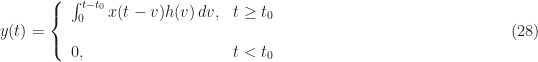
So causality requires the impulse response $h(t)$ to be zero for $t < 0$ , which makes sense because after all the impulse response is the system’s response to an impulse at $t = 0$ . The same requirement for causality is levied on the discrete-time impulse-response function $h(k)$ .

Stability

As we mentioned in the first part of this post, a system is bounded-input/bounded-output (BIBO) stable if every bounded input produces a bounded output. So for a bounded input $x(t)$ , there is some finite number $M_x$ such that

$\displaystyle |x(t)| < M_x \ \ \ \forall\ t \hfill(29)$

Another way of saying this is

$\displaystyle \max_t |x(t)| < M_x \hfill (30)$

Assuming we have a linear time-invariant system with impulse-response function $h(t)$ and output $y(t)$ , what is the condition on $h(t)$ for BIBO stability?

$\displaystyle y(t) = \int_{-\infty}^\infty x(u) h(t-u) \, du \hfill (31)$

$\displaystyle = \int_{-\infty}^\infty x(t-u) h(u) \, du \hfill (32)$

$\displaystyle \Rightarrow |y(t)| = \left| \int_{-\infty}^\infty x(t-u)h(u) \, du \right| \hfill (33)$

By elementary calculus, the magnitude of an integral is less than or equal to the integral of the integrand magnitude,

$\displaystyle |y(t)| \leq \int_{-\infty}^\infty | x(t-u) h(u)| \, du \hfill (34)$

$\displaystyle = \int_{-\infty}^\infty | x(t-u)|| h(u)| \, du \hfill (35)$

$\displaystyle \leq \int_{-\infty}^\infty M_x| h(u)| \, du \hfill (36)$

$\displaystyle = M_x \int_{-\infty}^\infty | h(u)| \, du \hfill (37)$

For $y(t)$ to be bounded, then, we require

$\displaystyle M_x \int_{-\infty}^\infty |h(u)| \, du < M_y \hfill (38)$

$\displaystyle \int_{-\infty}^\infty |h(u)| \, du < M_z < \infty \hfill (39)$

Equation (39) means that the impulse response is absolutely integrable. For discrete-time systems, the impulse-response function must be absolutely summable.

For a BIBO stable and causal linear time-invariant system, the requirement is

$\displaystyle \int_{0}^\infty |h(u)| \, du, < M_z < \infty \hfill (40)$

and a similar condition holds for the discrete-time impulse response $h(k)$ .

System Memory

For LTI systems, the memory of the system is the length of the non-zero portion of the impulse response. If there is some finite number $M$ for which $h(t) = 0$ for all $|t| > M$ , then the system is said to have finite memory.

In discrete time, a finite-memory linear shift-invariant system is also called a finite impulse response (FIR) filter. Otherwise, it is an infinite impulse response (IIR) filter. You can use MATLAB’s filter.m to implement FIR and IIR filters. Note that FIR filters are BIBO stable, IIR filters may or may not be. Why?

Significance of Linear Systems in CSP

We haven’t yet talked about the frequency-domain representation of a linear system (hint: it is the Fourier transform of the impulse-response function), so connecting LTI systems to CSP is a bit awkward at this point. However, LTI system models are prevalent in the modeling of communication-signal channels (for example, multipath propagation), and so we need to be able to understand how an LTI system that is applied to a signal affects the various CSP parameters of the filtered signal. We’ll be able to describe this mathematically more easily after we look at the frequency response of LTI systems. (For the impatient, go ahead and look at the post on signal processing operations Signal Processing Operations and CSP.)

When we talk about the spectral correlation function, we often speak of the temporal correlation between two “narrowband spectral components” of the signal. These narrowband spectral components are actually the outputs of two LTI systems (bandpass filters). We’ll get to the notions of lowpass, highpass, and bandpass filters in subsequent SPTK posts.

One application of CSP is source separation, in which the processed data contains two or more signals that overlap in both time and frequency, and the goal is to extract one or more of the signals from the noisy sum. A kind of signal separator that exploits CSP is known as the frequency-shift (FRESH) filter, which is a linear system, but it is not time-invariant. A FRESH filter is a multi-branch system where each branch consists of a frequency shifter followed by a FIR filter. We’ll eventualy have a post on FRESH filters at the CSP Blog.

Previous SPTK Post: The Fourier Transform Next SPTK Post: Frequency Response

Author: Chad Spooner

I'm a signal processing researcher specializing in cyclostationary signal processing (CSP) for communication signals. I hope to use this blog to help others with their cyclo-projects and to learn more about how CSP is being used and extended worldwide. View all posts by Chad Spooner

Laura on Blog Notes and Reader PollApril 1, 2023
Oops I meant just direction of arrival.
Laura on Blog Notes and Reader PollApril 1, 2023
Hi Chad! Adding to your probably lengthy list of topics to cover in your blog: a post on CSP for…
Chad Spooner on The Altar of OptimalityMarch 31, 2023
Yes, Sadok_mu, I think based on your comment, and your other comments, that we are "like-minded." Maybe neural networks will…
Chad Spooner on SPTK Addendum: Problems with resampling using MATLAB’s resample.mMarch 31, 2023
Thank you! I don't take any special action to reduce ringing or other distortions because I haven't seen the need.…
Chad Spooner on Blog Notes and Reader PollMarch 31, 2023
Then I should weight your response to the recent poll very very heavily indeed! Thanks!
Chad Spooner on The Altar of OptimalityMarch 31, 2023
You had me chuckling after reading this comment!
Dylan Gormley on Blog Notes and Reader PollMarch 31, 2023
I'm pretty sure 5,000 of those 7,145 views are me. Sorry for skewing the numbers.
Todd Reinking on The Altar of OptimalityMarch 31, 2023
Ha! This one had me chuckling until I shed a tear realizing that it summarized a lot of wasted hours…
SADOK_MU on The Altar of OptimalityMarch 30, 2023
Thank you professor for such deep thoughts. I agree that some paper produced is just useless and I'm against the…
Chad Spooner on Is Radio-Frequency Scene Analysis a Wicked Problem?March 30, 2023
More from Conklin (The Literature [R186]): three forces that fragment projects just as surely as rain creates mud: wicked problems,…