
In this post, I show the non-conjugate and conjugate spectral correlation functions (SCFs) for the rectangular-pulse BPSK signal we generated in a previous post. The theoretical SCF can be analytically determined for a rectangular-pulse BPSK signal with independent and identically distributed bits (see My Papers [6] for example or The Literature [R1]). The cycle frequencies are, of course, equal to those for the CAF for rectangular-pulse BPSK. In particular, for the non-conjugate SCF, we have cycle frequencies of 


The simulated BPSK signal is used as input to the frequency-smoothing method of spectral correlation estimation (My Papers [6], The Literature [R1, R5]). The signal has bit rate of 


Only the non-negative cycle frequencies are shown for the non-conjugate SCF due to symmetry of the SCF.
The theoretical SCF formula can be numerically evaluated using the parameters of our rectangular-pulse BPSK signal, and the result is plotted below:

The match is excellent!
At this point at the CSP Blog, we have generated a useful test signal, defined the basic temporal and spectral second-order parameters of cyclostationary signals, and shown that our formulas and estimates match for the test signal. We are prepared to begin study of more complex mathematical topics and, perhaps most usefully, study of the cyclostationarity properties of sophisticated real-world signals.
Comparison to a Bandwidth-Efficient BPSK Signal
The rectangular-pulse BPSK signal has infinite bandwidth, and so theoretically has an infinite number of cycle frequencies. But most of them correspond to spectral correlation functions with very small maximum magnitudes. Most BPSK signals we’re likely to encounter in practice will be bandwidth-efficient signals, meaning their occupied bandwidth is not more than twice their symbol rate. A common pulse function is the square-root raised-cosine pulse, which is characterized by the pulse roll-off parameter ![r \in [0, 1]](https://s0.wp.com/latex.php?latex=r+%5Cin+%5B0%2C+1%5D&bg=ffffff&fg=1a1a1a&s=0&c=20201002)


Here, we’ll just compare to a single SRRC BPSK signal with 

Can you post the matlab code to plot these figures ?
Sorry for the late reply. The code that plots my SCFs and CAFs strongly depends, of course, on the format of the SCF or CAF to be plotted. We haven’t covered estimators yet. But if you can get your estimates or ideal functions in matrix form, so that each SCF estimate, for example, corresponds to all frequencies [-0.5, 0.5) regardless of the value of cycle frequency, then you can use waterfall.m in MATLAB to get plots similar to mine:
h = waterfall (fnc(1:subsamp:end)*fs/fsFac + fcarrier/fsFac, …
anc*fs/asFac, …
((abs(ync(:, 1:subsamp:end)))), zeros(size(ync(:, 1:subsamp:end))));
set (h, ‘edgecolor’, [0 0 0]);
set (h, ‘facecolor’, [0.9 0.9 0.95]);
grid on;
axis tight;
xlabel (‘f (Hz)’);
ylabel (‘\alpha (Hz)’);
Here fnc is the frequency vector, anc is the cycle-frequency vector, and the function to be plotted is the matrix ync. The extra zeros in the waterfall.m call force the color of the edges to be black, then I color the faces with the set() calls.
The subsamp integer controls how much I subsample the various functions, which is usually needed because MATLAB takes a long time to plot the surface if the sizes of fnc and anc are large.
I usually have to play around with the viewing angle when doing three-dimensional plots. For these plots I used
view (-150, 30);
Does that help?
Ok, I will try this way . So do you think that the method showed in the link will be useful http://www.mathworks.com/examples/matlab-communications/2875-p25-spectrum-sensing-with-synthesized-and-captured-data#2
using the case “Non-P25 Signal Case with Synthesized Data”
Hi Chad, Thank you for your blog. Here you mentioned that a rectangular pulse has infinite bandwidth. My question is only somewhat relevant but I thought I could use your help. I am interested in what happens to the autocorrelation of a random process when it is passed through a Heaviside step function. In other words, how is the autocorrelation of the input noise related to the autocorrelation of the output rectangular binary waveform.
I found a relationship for the mean-squared bandwidths when a correlated random processes is transmitted through a nonlinearity in equation 11 of this paper: https://ieeexplore.ieee.org/abstract/document/1054033
Namely, this equation relates the mean-squared bandwidth of the output process to that of the input process. However, the term g’^2, where g’ is the derivative of the nonlinearity, is problematic given that the derivative of the step function is the dirac delta function and we end up with the delta function squared (maybe this is a consequence of the fact that a rectangular waveform has infinite bandwidth, as you pointed out).
Do you by any chance know how one can relate the autocorrelation function of a stochastic process to the autocorrelation of a rectangular waveform which is created by applying the Heaviside step function at every point of the input stochastic process?
Many thanks for your help!
Riemannk: Thanks so much for stopping by the CSP Blog!
I think we can get close to an answer to your question, but first I think it is not sufficiently precise. In particular, can you please define “is passed through a Heaviside step function.” “passed through” is not clear. I have an idea of what you mean, but I don’t want to go with it until I’m sure. If it is more convenient to describe what you mean using pictures, go ahead and email me at cmspooner@ieee.org and I’ll insert them in this comment thread. I can’t get WordPress to allow readers to add images to comments … yet. Some people post their pictures to imgur.com, but I’m happy to insert here.
Hi Chad
Why is the region of support in the bifrequency plane for the theoretical spectral correlation surfaces for a rectangular-pulse BPSK signal not the diamond region? While the frequency-smoothing method of spectral correlation estimation of the rectangular-pulse BPSK signal is the diamond region.
On the other hand, a rectangular-pulse BPSK signal is a band-pass signal. So there should be four diamond region in the bifrequency plane. It means that you did not plot all regions, right?
I’ve updated the post to add captions to the figures. I think you are asking why the diamond-shaped principal domain for the spectral correlation function is not visible in the theoretical plots of Figure 2, but it is visible in the estimated plots of Figure 1. The reason is that the theoretical surfaces arise from the numerical evaluation of a spectral correlation function formula for a continuous-time BPSK signal, and so the formula is valid for all and
and  –there is no principal domain in continuous time.
I use complex-valued signals in the CSP blog. So, no, the signal I’m processing here is not a bandpass signal. It is a low-pass complex-envelope signal. Instead of four diamonds in the –
– plane, we use two separate planes: the non-conjugate and conjugate.
Hi Dr. Spooner,
First, thanks for putting this blog together. I’m just getting started with cyclostationary signal analysis and it’s been very helpful (I’m interested in using it to automatically identify human-made radio frequency interference in radio astronomy signals). I’m trying to go through the beginner posts and reproduce some of your plots by coding things up in python. I’m getting close with some of my approaches, but there my results differ from yours in ways I don’t totally understand. I know you don’t do direct help with code, but I was wondering any of my descriptions (I’m not sure how to post figures in the comments) might lead you to suspect some specific error that I can explore on my own.
First, all of these results are using a rectangular pulse BPSK signal that I am generating via a port of your Matlab code to python. In normalized units, I am generating a signal of 4000 bits, with a bit-rate of 0.1 and carrier frequency of 0.05. The plots below don’t include any additive noise. I think I’m doing this correctly, but I haven’t used Matlab so it’s possible I translated something incorrectly. But assuming it is correct, here are some of my results.
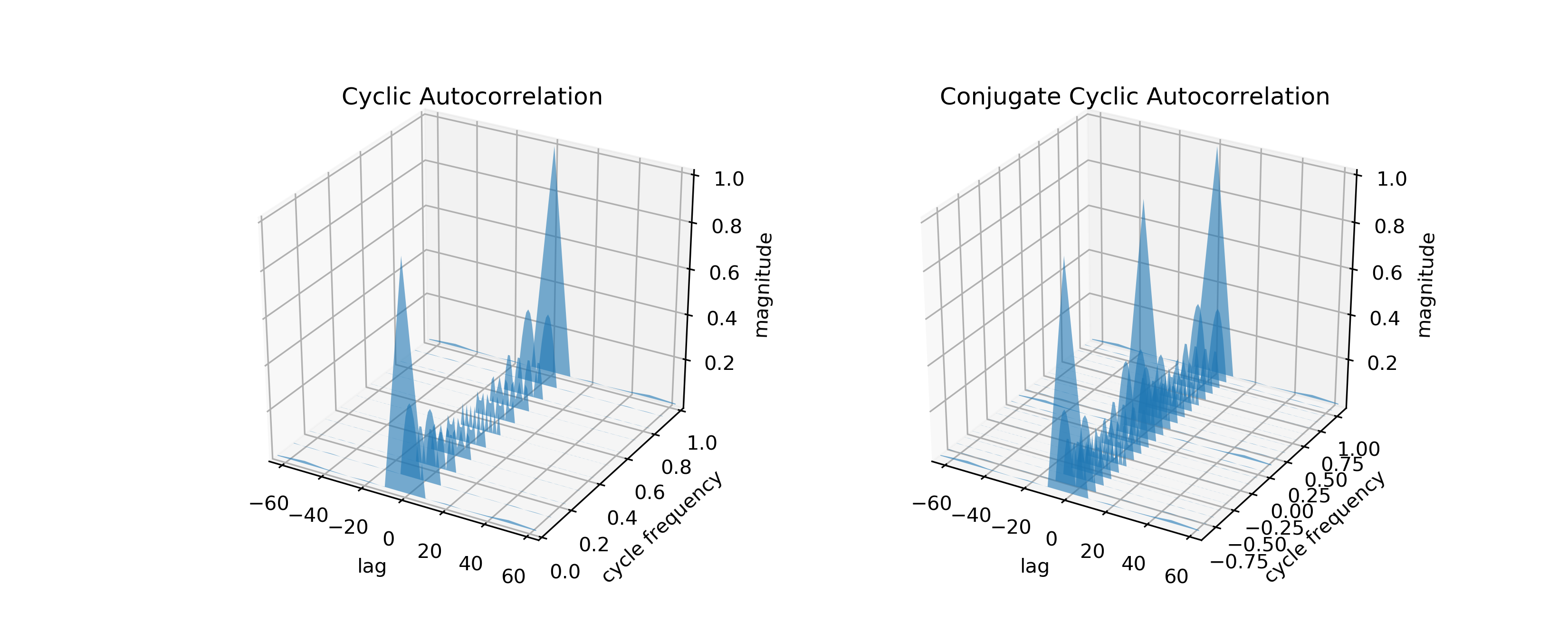
First I try to directly compute the cyclic and conjugate cyclic autocorrelation functions. I notice two differences in my results and yours. First, the magnitude of the correlation coefficients don’t decay away in my results as quickly as in yours. Second, the correlation coefficients start to repeat at higher cycle frequencies, specifically at a (normalized) cycle frequency of 1.0 for my example above (i.e. the CAF at a cycle frequency of 0 seems almost identical to that at 1.0).
Next, I tried to take the FFT (using the numpy FFT module) of the above autocorrelation functions to see if I could reproduce the spectral and conjugate spectral correlation functions following the W-K theorem. Of course, I see the signal repeat at higher cycle frequencies again. I’m also not seeing peaks in the correlation function at positive Fourier frequencies, as I would expect (i.e., I dont see the “V” shape in your plots). Instead the significant peaks run at a diagonal.
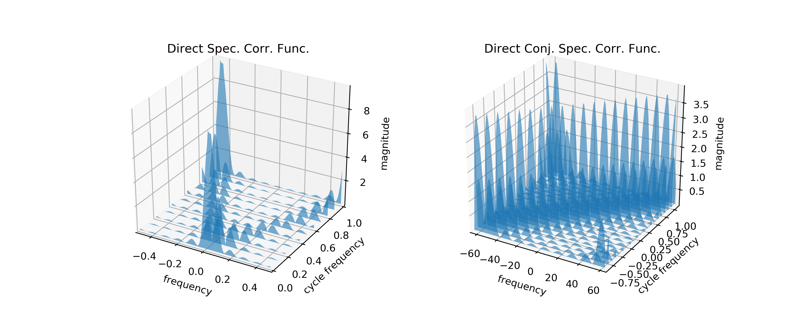
Finally, I tried to directly compute the spectral and conjugate spectral correlation function, i.e. I’m trying to average the cyclic and conjugate cyclic periodograms rather than use the W-K theorem.
The spectral correlation function looks reasonable, i.e. I see the “V” shape, but I also see the magnitude increase again at high cycle frequencies. The conjugate spectral correlation function looks very different from your results, though. I see a only diagonal feature instead of the “X” feature.
I’m happy to post the python code if you would like, but as I said, I realize you prefer not to debug code directly. But in words, here is what I am trying to do.
For the CAF
1) I create the RP BPSK signal
2) For each lag, I use the numpy.roll function to rotate the signal by the lag value. I then multiply this rotated signal by the conjugate of the un-rotated signal by exp(-2j*pi*cf*ts), where ts is just the indices of the signal array (i.e. numpy.arange(len(x))), and then I average this.
For the CCAF, it’s the same, except I don’t take the conjugate of the un-rotated signal.
For W-K theorem approach to the SCF and CSFC, I just take the FFT using numpy.fft.fft along the lag axes.
For the direct SCF
1) I generate the RP BPSK signal
2) For each cycle frequency, I multiply one copy of this time-domain signal by exp(2j*pi*cf/2*t) and second copy by exp(-2j*pi*cf/2*t), where cf is the cycle frequency. That is, I use the frequency shift property of the FT to shift by the cycle frequencies. Call these x1 and x2.
3) For each time sample, I then take a sliding window FFT of some window size (equal to the number of lags used above) that starts at that time sample (call these X1 and X2). I then take the average of X1 *conjugate(X2).
For the CSCF, it is very similar.
1) I generate the RP BPSK signal
2) For each cycle frequency, I multiply one copy of this time-domain signal by exp(2j*pi*cf/2*t) and second copy by exp(-2j*pi*cf/2*t), where cf is the cycle frequency. That is, I use the frequency shift property of the FT to shift by the cycle frequencies. Call these x1 and x2. I then take the conjugate of x2. I think this should shift the frequency of x2 to -f + cf/2.
3) For each time sample, I then take a sliding window FFT of some window size (equal to the number of lags used above) that starts at that time sample (call these X1 and X2). I then take the average of X1 *conjugate(X2).
Thanks for putting up with this long post, and again, thanks for the blog. I’m happy to share figures if there is some way to do that.
Cyclic Autocorrelation Estimates:
Fourier Transformed Cyclic Autocorrelation Estimates:

Spectral Correlation Estimates:
Ryan: Thank you for visiting the CSP Blog and providing us all with your current status on do-it-yourself CSP. I really appreciate this kind of comment, and I know it helps others as well.
I’ve added the images you sent to me by email. WordPress does not allow commenters to add images.
I think you are on the right track. In the time domain, not only do we have to make sure that our data is adequately sampled, but we have to make sure that the complex sine wave (multiplying the delay product) is adequately sampled. This means that we might not be able to unambiguously represent the complex sine wave for all cycle frequencies of interest, forcing us to increase the sampling rate if we want to stick with the straightforward time-domain estimate of the cyclic autocorrelation.
Hello,
nice blog dr.Spooner. I just want to ask if Im on right way to achieve SCF and then CAF from SCF or the way how can I be sure I have done proposed functions successfully. I used BPSK signal with same parameters as yours BPSK proposed in blog but in my opinion I have different plots than yours. I tried to attach here my code in Matlab to txt but unsuccessfully. Thank you for your response.
Here is my code:
clc;
clear all
close all
%%%%%%%%%%%%
M = 2;
Fs = 1;
n_bit = 4000;
Fb = 0.1;
spb = Fs/Fb;
fSpan = 2;
time = 0:1:n_bit-1;
freq = 0:1/(n_bit-1):1;
N_psd = 1024;
%%%%%%%%%%%%
data = randi([0 M-1],n_bit,1);
dmodData = (pskmod(data,M));
txFilter = comm.RaisedCosineTransmitFilter(“Shape”,”Square root”,”RolloffFactor”,0.3,”FilterSpanInSymbols”,fSpan,”OutputSamplesPerSymbol”,spb);
txfilterOut = txFilter(dmodData)’;
time = 0:1:length(txfilterOut)-1;
freq = 0:1/(length(txfilterOut)-1):1;
figure(1)
plot(time,real(txfilterOut),’r’)
hold on
plot(time,imag(txfilterOut),’b’)
title(‘time domain’)
spek = fftshift(abs(fft(txfilterOut)));
figure(2)
plot(freq,spek)
title(‘freq. domain’)
num_blocks = floor(length(txfilterOut) / N_psd);
S = txfilterOut(1, 1:(N_psd*num_blocks));
S = reshape(S, N_psd, num_blocks);
I = fft(S);
I = I .* conj(I);
I = sum(I.’);
I = fftshift(I);
I = I /(num_blocks * N_psd);
freq_c = [0:(N_psd-1)]/N_psd – 0.5;
figure(3)
plot(freq_c,10*log10(I))
title(‘PSD’)
num_blocks = floor(length(txfilterOut) / N_psd);
alpha = 0:0.1:0.5;
for i = 1:length(alpha)
txfilterOutte = txfilterOut(1, 1:(N_psd*num_blocks));
modulplu = txfilterOutte.*exp(1j*2*pi*alpha(1,i)/2.*[1:(N_psd*num_blocks)]);
modulminu = txfilterOutte.*exp(1j*2*pi*-alpha(1,i)/2.*[1:(N_psd*num_blocks)]);
modulplu = reshape(modulplu, N_psd, num_blocks);
modulminu= reshape(modulminu, N_psd, num_blocks);
x1 = fft(modulplu);
x2 = fft(modulminu);
I = x1 .* conj(x2);
Isum = sum(I.’);
Isum = fftshift(Isum);
Iabsft(i,:) = Isum /(num_blocks * N_psd);
end
freq_c = [0:(N_psd-1)]/N_psd – 0.5;
[alko,tauco] = meshgrid(alpha,freq_c);
figure(4)
plot3(tauco,alko,10*log10(Iabsft))
xlabel(‘f’)
ylabel(‘\alpha’)
zlabel(‘S(f)\alpha [dB]’)
title(‘SCF’)
CAFtry = [];
for i = 1:length(alpha)
CAFtry(i,:) = abs(fftshift(ifft(Iabsft(i,:))));
end
time_c = linspace(-n_bit/2,n_bit/2,N_psd);
[alko,tauco] = meshgrid(alpha,time_c);
figure(5)
plot3(tauco,alko,CAFtry)
xlabel(‘\tau’)
ylabel(‘\alpha’)
zlabel(‘R(t)\alpha’)
title(‘CAF’)
Thanks for reading the CSP Blog, Temugin, and for the comment!
It looks to me, so far, like you are on the right track.
You are replying to the post on the spectral correlation function for rectangular-pulse BPSK signals, but you simulated a square-root raised-cosine BPSK signal. So the plots will look quite different. In particular, the SRRC BPSK signal has only three non-conjugate cycle frequencies: , which for you will be
  and it is safe to ignore the negative non-conjugate cycle frequencies due to symmetry (as you are doing). Rectangular-pulse BPSK, on the other hand, has an infinite number of cycle frequencies, and certainly the first ten or so produce readily identifiable spectral correlation shapes. They get small after that.
Also, if you want to plot the spectral correlation estimates, it is best to plot their magnitude, and definitely take the absolute value before converting to decibels as in