Cyclic Temporal Cumulants

Cyclic cumulants are the amplitudes of the Fourier-series components of the time-varying cumulant function for a cyclostationary signal. They degenerate to conventional cumulants when the signal is stationary.

In this post I continue the development of the theory of higher-order cyclostationarity (My Papers [5,6]) that I began here. It is largely taken from my doctoral work (download my dissertation here).

This is a long post. To make it worthwhile, I’ve placed some movies of cyclic-cumulant estimates at the end. Or just skip to the end now if you’re impatient!

In my work on cyclostationary signal processing (CSP), the most useful tools are those for estimating second-order statistics, such as the cyclic autocorrelation, spectral correlation function, and spectral coherence function. However, as we discussed in the post on Textbook Signals, there are some situations (perhaps only academic; see my question in the Textbook post) for which higher-order cyclostationarity is required. In particular, a probabilistic approach to blind modulation recognition for ideal (textbook) digital QAM, PSK, and CPM requires higher-order cyclostationarity because such signals have similar or identical spectral correlation functions and PSDs. (Other high-SNR non-probabilistic approaches can still work, such as blind constellation extraction.)

Recall that in the post introducing higher-order cyclostationarity, I mentioned that one encounters a bit of a puzzle when attempting to generalize experience with second-order cyclostationarity to higher orders. This is the puzzle of pure sine waves (My Papers [5]). Let’s look at pure and impure sine waves, and see how they lead to the probabilistic parameters widely known as cyclic cumulants.

Sine Waves Times Sine Waves Equals Sine Waves

Suppose we have a single complex-valued sine wave given by

$\displaystyle x(t) = A_0e^{i2\pi f_0 t + i \phi_0}, \hfill (1)$

where $A_0$ is the amplitude, $f_0$ is the frequency, and $\phi_0$ is the phase. If we consider a quadratic operation on this signal to produce the signal $y(t)$ , we will find another sine wave,

$\displaystyle y(t) = x(t+\tau_1) x(t+\tau_2) = A_0^2 \ e^{i2\pi 2f_0 t + i2\phi_0} e^{i2\pi f_0 (\tau_1 + \tau_2)}. \hfill (2)$

That is, this particular quadratic operation leads to a sine wave with frequency $2f_0,$ phase $2\phi_0 + 2\pi f_0 (\tau_1 + \tau_2)$ , and complex amplitude $A_0^2$ . If we had included a conjugation on the second factor, $x^*(t+\tau_2)$ , the result is a trivial sine wave with zero frequency, amplitude $|A_0|^2$ , and phase depending on $\tau_1$ and $\tau_2$ .

Next consider a signal consisting of the sum of two sine waves with different frequencies,

$\displaystyle x(t) = A_0 e^{i2\pi f_0 t + i\phi_0} + A_1e^{i2\pi f_1 t + i\phi_1}. \hfill (3)$

The simple (no-conjugate) second-order operation $x(t+\tau_1)x(t+\tau_2)$ leads to

$\displaystyle y(t) = A_0^2 e^{i2\pi 2f_0 t + 2i\phi_0 + i2\pi f_0(\tau_1 + \tau_2)}$

$\displaystyle + A_1^2 e^{i2\pi 2f_1 t + 2\phi_1 + i 2 \pi f_1(\tau_1 + \tau_2)}$

$\displaystyle + 2A_0 A_1 e^{i2\pi (f_0 + f_1)t + i(\phi_0 + \phi_1)} \hfill (4)$

In other words, the quadratic transformation to $y(t)$ leads to sine-wave components with frequencies of $2f_0$ , $2f_1$ , and $f_0 + f_1$ . Other quadratic operations, such as those with a single conjugated factor or two conjugated factors, lead to different sine-wave frequencies in $y(t)$ , but they all produce at least one sine-wave component.

Impure Sine Waves

Now recall that our working definition of cyclostationarity is that at least one non-trivial sine wave can be generated by subjecting the signal of interest to a quadratic nonlinearity, even when the signal itself contains no such sine-wave component. So how does the previous discussion of `sine waves begetting sine waves’ apply?

A natural extension of second-order theory to higher orders is to simply increase the order of the moment that we considered when defining the cyclic autocorrelation function. The usual second-order lag product

$\displaystyle x(t+\tau/2)x^*(t-\tau/2)$

can be generalized to

$\displaystyle x(t + \tau_1)x^*(t + \tau_2)$

and then we could consider the third-order or fourth-order versions

$\displaystyle x(t+\tau_1) x^*(t+\tau_2) x(t+\tau_3)$

and

$\displaystyle x(t+\tau_1)x^*(t+\tau_2) x(t+\tau_3) x^*(t+\tau_4)$ .

It turns out that the odd-order moments are zero for almost all communication signals, so going forward we’ll consider only even-order moments, such as the moment corresponding to the fourth-order lag product. That is, we consider the expected value of the lag product,

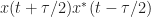
$\displaystyle R_x(t, \boldsymbol{\tau}; 4) = E \left[x(t+\tau_1)x^*(t+\tau_2) x(t+\tau_3) x^*(t+\tau_4)\right]. \hfill (5)$

We know that this fourth-order moment contains sine-wave components because the second-order lag product $x(t+\tau_1)x^*(t+\tau_2)$ contains sine waves, the second-order lag product $x(t+\tau_3)x^*(t+\tau_4)$ contains sine waves, and sine waves multiplied by sine waves results in sine waves. In particular, suppose $x(t)$ possesses a second-order non-conjugate cycle frequency $\alpha$ when the lags are $\tau_1$ and $\tau_2$ . It also must possess the non-conjugate second-order cycle frequency of zero (it possesses power), so that the sine wave with frequency $\alpha$ in $x(t+\tau_1)x^*(t+\tau_2)$ multiplies the sine wave with frequency zero in $x(t+\tau_3)x^*(t+\tau_4)$ , producing a sine wave with frequency $\alpha$ in the fourth-order lag product (for suitable values of $\tau_3$ and $\tau_4$ , such as zero).

This kind of analysis can be performed for other choices of conjugations and lag-vector values $\tau_i$ . The conclusion is that the sine-wave components in a higher-order lag product are due, at least in part, to the interactions between lower-order sine-wave components, because `sine waves times sine waves equals sine waves.’ So is there a component of any of the fourth-order sine waves that is NOT due to these lower-order interactions?

We’ll call the sine waves in the lag product (the moment sine waves) impure sine waves, because they will often contain products of lower-order components. Any component of the impure sine waves that does not arise from the interactions of the lower-order sine waves will be called a pure sine wave.

Purifying Sine Waves

To purify the impure sine waves in some $n$ th-order lag product, we’ll need to identify the impure culprits and subtract them. Let’s start with a simple case where the signal itself does, in fact, contain additive sine-wave components. Then the second-order lag product must contain sine waves, and we can set about purifying the second-order lag product, which simplifies our notation. Then we’ll extend the ideas to higher-order lag products.

Suppose our signal $x(t)$ consists of our old friend the rectangular-pulse BPSK signal plus an additive sine-wave component

$\displaystyle x(t) = s_{bpsk}(t) + A_0 e^{i2\pi 0.05 t + i\phi_0} + A_1 e^{i2\pi (-0.05) t + i\phi_1}. \hfill (6)$

Recall that the BPSK signal has a symbol rate of $0.1$ and a carrier frequency of $0.05$ (normalized-frequency parameters). If we consider the non-conjugate cycle frequencies of $x(t)$ , we see that the BPSK signal contributes the bit-rate harmonics $\alpha_{bpsk} = k/T_0 = 0.1k$ , and that the two sine sine waves contribute $\alpha_{sine} = \{0, 0.1, -0.1\}$ . For the conjugate cycle frequencies, the BPSK signal contributes

$\displaystyle \beta_{bpsk} = 2f_c + k/T_0 = 0.1 + 0.1k = \{\ldots, -0.5, -0.4, \ldots, 0.3, 0.4, 0.5, \ldots \}, \hfill (7)$

and the sine waves contribute $\beta_{sine} = \{0, 0.1, -0.1\}$ . Therefore, for both the non-conjugate and conjugate cases, the BPSK and sine wave share cycle frequencies. However, only the BPSK signal produces second-order sine-wave components that are not the result of products of first-order sine waves.

One way to proceed with the purification in this case is to just subtract off the sine waves from $x(t)$ and then compute the cyclic autocorrelation or spectral correlation function of the result. But that method doesn’t generalize well to the case where there are no first-order sine waves. So let’s take a more systematic approach.

The lower-order (first-order) sine wave frequencies are $\pm 0.05$ , and the sine-wave created frequencies in the second-order lag product are $\{0, 0.1, -0.1\}$ . Considering the non-conjugate second-order cycle frequency of 0, we see that it has a component due to the BPSK signal and a component due to the tones. If the lag product in question is

$\displaystyle L_x(t, \boldsymbol{\tau}; 2, 1) = x(t+\tau_1)x^*(t+\tau_2), \hfill (8)$

then the sine-wave induced component has complex amplitude

$\displaystyle |A_0|^2 e^{i2\pi 0.05 (\tau_1 - \tau_2)} + |A_1|^2 e^{-i2\pi 0.05 (\tau_1 - \tau_2)}. \hfill (9)$

This is just the sum of the complex amplitudes for each sine wave multiplied by itself. So if we extract the zero-frequency sine wave from the second-order lag product, and then subtract from it the complex amplitude of each unique product of first-order sine waves with resultant frequency zero, we’ll be left with the complex amplitude due solely to the BPSK signal. The lower-order product terms will be removed, and we’ll have purified the second-order sine wave:

$P_x(\boldsymbol{\tau}; 2, 1) = \left\langle L_x(t, \boldsymbol{\tau}; 2, 1) e^{i 2 \pi 0 t} \right\rangle - \left\langle x(t+\tau_1)e^{i 2 \pi 0.05 t} \right\rangle \left\langle x^*(t+\tau_2)e^{i 2 \pi (-0.05) t} \right\rangle$

$\displaystyle - \left\langle x(t+\tau_1)e^{i2\pi (-0.05) t} \right\rangle \left\langle x^*(t+\tau_2) e^{i2\pi 0.05 t} \right\rangle. \hfill (10)$

The idea is to subtract all unique products of the lower-order sine waves such that the sum of the sine-wave frequencies for each product is equal to the specified second-order cycle frequency. Here we are targeting the second-order cycle frequency of $0$ , so we subtract the product of first-order sine waves with frequencies $0.05$ (in $x(t+\tau_1)$ ) and $-0.05$ (in $x^*(t+\tau_2)$ ), and also the product with frequencies $-0.05$ (in $x(t+\tau_1)$ ) and $0.05$ (in $x^*(t+\tau_2)$ ).

Suppose the signal $x(t)$ actually contained $K$ sine-wave components with frequencies $\{f_k\}_{k=1}^K$ . Let the second-order non-conjugate cycle frequency of interest be $\alpha$ . Then we seek to subtract off lower-order products for each pair of frequencies $f_1$ and $F_2$ such that

$F_1 + (-)F_2 = \alpha. \hfill (11)$

In our example above, the frequency set is $\{0.05, -0.05\}$ and $\alpha = 0$ . Then we have the two sets of pairs $(0.05, 0.05)$ and $(-0.05, -0.05)$ . For $\alpha = 0.1$ , we have the single pair $(0.05, -0.05)$ , which makes sense because there is only one product of sine waves that has frequency $0.1$ , and that is the sine wave with frequency $0.05$ in the unconjugated (first) factor, and $-0.05$ in the conjugated factor.

Partitions of the Index Set $\{1, 2, \ldots, n\}$

A key phrase in the development above is “unique products of lower-order sine waves.” How do we characterize such unique products? For the general case of an $n$ th-order moment, we are thinking about the sine-wave components of the $n$ th-order lag product

$\displaystyle L_x(t, \boldsymbol{\tau};n,m) = \displaystyle \prod_{j=1}^n x^{(*)_j}(t+\tau_j), \hfill (12)$

where $(*)_j$ denotes an optional conjugation, and there are $m$ factors that are conjugated. We want to account for every possible product of lower-order sine waves whose frequencies sum to the cycle frequency of interest $\alpha$ . So there could be a sine wave in $x^{(*)_1}(t+\tau_1) x^{(*)_2}x(t+\tau_2)$ that multiplies a sine wave in $x^{(*)_3}(t+\tau_3) \ldots x^{(*)_n}(t+\tau_n)$ and whose sum is $\alpha$ , and maybe a sine wave in $x^{(*)_1}(t+\tau_1) x^{(*)_3}(t+\tau_3)x^{(*)_5}(t+\tau_5)$ that multiplies a sine wave in $x^{(*)_2}(t+\tau_2) x^{(*)_4}(t+\tau_4)x^{(*)_6}(t+\tau_6) \ldots x^{(*)_n}(t+\tau_n)$ , or possibly any other partitioning of the $n$ involved factors $x^{(*)_j}(t+\tau_j)$ .

So we have to consider all the ways of partitioning the set of factors, and then for each one of these partitions, we have to determine whether or not the lag products for the partitions contain sine-wave components that sum to the desired cycle frequency $\alpha$ . Whew. That is indeed complicated.

But the purification idea leads to the idea of partitions of a set of $n$ elements, in this case the $n$ elements $x^{(*)_j}(t+\tau_j)$ . For simplicity, we can associate these elements with the index set $I_n = \{1, 2, \ldots, n\}$ . A partition of $I_n$ is a collection of proper subsets $\{\nu_k\}_{k=1}^p$ whose union is $I_n$ and whose pairwise intersections are all the empty set. This is just what we need to characterize all the possible ways lower-order sine waves can combine to contribute to the lag-product sine wave.

For $n=2$ , we have $I_2 = {1, 2}$ and the partitions are

$q_1 = \{1, 2\}; p = 1 \hfill (13)$

$q_2 = \{\{1\}, \{2\}\}; p = 2 \hfill (14)$

and there are no others (no unique partitions, anyway, because $\{\{2\}, \{1\}\}$ is not unique). For $n=3$ , the partitions are

$q_1 = \{1, 2, 3\}; p = 1 \hfill (15)$

$q_2 = \{\{1\}, \{2, 3\}\}; p = 2 \hfill (16)$

$q_3 = \{\{2\}, \{1, 3\}\}; p = 2 \hfill (17)$

$q_4 = \{\{3\}, \{1, 2\}\}; p = 2 \hfill (18)$

and

$q_5 = \{\{1\}, \{2\}, \{3\}\}; p = 3 \hfill (19)$

The number of partitions rapidly increases with the index size $n$ . (The number of partitions is given by Bell’s number, which makes use of Stirling numbers of the second kind.) For example, there are $15$ partitions for $n=4$ ,

Fortunately, any partitions containing any element that has an odd size, such as a singleton $\{3\}$ or a three-element set $\{2, 3, 4\}$ can usually be ignored in the computation of a pure sine wave because the signal under study has no first-order sine-wave components nor any non-zero odd-order moments. So, typically for $n=4$ , the partitions that matter are only

$\{1, 2, 3, 4\}$

$\{\{1, 2\}, \{3, 4\}\}$

$\{\{1, 3\}, \{2, 4\}\}$

$\{\{1, 4\}, \{2, 3\}\}$

The partitions of $I_n$ can be easily computed recursively.

Getting back to purifying sine waves, we have arrived at the idea that to find the pure sine-wave component of some $n$ th-order lag product, we need to subtract from that lag product all products of lower-order sine-wave components that have frequencies that sum to the desired frequency, and this can be done by using the partitions of the index set. To ensure that we don’t end up subtracting off the same sine wave component multiple times, we wish to subtract from the lag product all products of lower-order pure sine-wave components.

We can get all the pure $n$ th order sine waves at once by subtracting all the products of pure lower-order sine waves from the sum of all $n$ th-order sine waves. That is, let $E^\alpha[\cdot]$ represent the general sine-wave extraction operator,

$\displaystyle E^\alpha[x(t)] = \sum_{\beta} \left\langle x(t) e^{-i2\pi\beta t} \right\rangle e^{i2\pi\beta t}, \hfill (20)$

where the sum is over all frequencies $\beta$ for which the signal $x(t)$ contains a sine-wave component with non-zero amplitude,

$\left\langle x(t) e^{-i2\pi\beta t} \right\rangle \neq 0. \hfill (21)$

In other words, $E^\alpha [\cdot]$ extracts all the impure sine waves from its argument.

Our purified sine waves are then given by

$\displaystyle P_x(t,\boldsymbol{\tau}; n,m) = E^\alpha[L_x(t,\boldsymbol{\tau};n,m)] - \sum_{P,\, p\neq 1} \prod_{j=1}^p P_x(t,\boldsymbol{\tau_j}; n_j, m_j), \hfill (22)$

where the sum is over all $n$ th-order partitions of the index set $I_n$ , and each partition has size $2 \leq p \leq n$ with elements $\{\nu_j\}_{j=1}^p$ having sizes $|\nu_j| = n_j$ and numbers of optional conjugations $m_j$ .

The Shiryaev-Leonov Moment-Cumulant Formula

In the theory of random variables and processes, the $n$ th-order moment function is defined as the expected value of the product of $n$ variables. For simplicity, let’s consider $n$ random variables $X_j$ for $j=1, 2, \ldots, n$ . Then the $n$ th-order moment is

$\displaystyle R_{\boldsymbol X} (n) = E[\prod_{j=1}^n X_j]. \hfill (23)$

The moment also appears in the series expansion of the characteristic function,

$\displaystyle \Phi_{\boldsymbol X} (\boldsymbol{\omega}) = E\left[e^{i\boldsymbol{\omega}^\prime {\boldsymbol X}}\right], \hfill (24)$

which we won’t get into here. However, the cumulants appear in the series expansion of the logarithm of the characteristic function. With the moments, we can directly compute the value by time or ensemble averaging in practice, but how do we compute cumulants (leaving aside for now why we would even want to, but see this post if you can’t help yourself)? Fortunately for us, the relationship between the $n$ th-order moment and the $n$ th-order cumulant was derived long ago, by Shiryaev and Leonov (My Papers [13], Downloads).

The $n$ th-order cumulant is given by a nonlinear combination of lower-order moments,

$\displaystyle C_{\boldsymbol X} (n) = \sum_P \left[ (-1)^{p-1} (p-1)! \prod_{j=1}^p R_{{\boldsymbol X}_j} (n_j) \right], \hfill (25)$

where the sum is over all unique partitions $P$ of the index set $I_n$ , each having $p$ elements $\{\nu_j\}_{j=1}^p$ . The notation ${\boldsymbol X}_j$ indicates the $n_j = |\nu_j|$ elements $\{X_k: k \in \nu_j\}$ . The reverse formula, that gives the moment in terms of the lower-order cumulants is

$\displaystyle R_{\boldsymbol X} (n) = \sum_P \left[ \prod_{j=1}^p C_{{\boldsymbol X}_j} (n_j) \right], \hfill (26)$

which should look familiar. It is the same formula as the pure-sines-waves formula. To see this more clearly, break up the sum over the partitions into one term for $p = 1$ and one term for all the other partitions,

$\displaystyle R_{\boldsymbol X} (n) = C_{\boldsymbol X} (n) + \sum_{P,\, p\neq 1} \left[ \prod_{j=1}^p C_{{\boldsymbol X}_j} (n_j) \right], \hfill (27)$

$\displaystyle C_{\boldsymbol X} (n) = R_{\boldsymbol X} (n) - \sum_{P, \, p\neq 1} \left[ \prod_{j=1}^p C_{{\boldsymbol X}_j} (n_j) \right]. \hfill (28)$

Cyclic Cumulants

The $n$ th-order temporal moment function is simply

$\displaystyle R_x(t, \boldsymbol{\tau};n,m) = E^\alpha \left[ \prod_{j=1}^n x^{(*)_j}(t+\tau_j) \right], \hfill (29)$

and the $n$ th-order cyclic temporal moment function is a Fourier coefficient of the (poly)periodic moment,

$R_x^\alpha(\boldsymbol{\tau};n,m) = \left\langle R_x(t,\boldsymbol{\tau};n,m) e^{-i2\pi \alpha t} \right\rangle. \hfill (30)$

The $n$ th-order temporal cumulant function is given by the now-familiar combination of products of lower-order temporal moment functions,

$\displaystyle C_x (t, \boldsymbol{\tau};n,m) = \sum_{P} \left[ (-1)^{p-1}(p-1)! \prod_{j=1}^p R_x(t, \boldsymbol{\tau}_j; n_j, m_j) \right]. \hfill (31)$

Now the $n$ th-order cyclic temporal cumulant function (cyclic cumulant) is just a Fourier coefficient of the temporal cumulant function

$\displaystyle C_x^\alpha (\boldsymbol{\tau}; n,m) = \sum_{P} \left[ (-1)^{p-1}(p-1)! \sum_{\boldsymbol{\beta}^\dagger \boldsymbol{1}=\alpha} \prod_{j=1}^p R_x^{\beta_j} (\boldsymbol{\tau}_j; n_j, m_j) \right]. \hfill (32)$

The vector of cycle frequencies $\boldsymbol{\beta} = [\beta_1\ \beta_2 \ \ldots \beta_p]$ is the vector of cyclic temporal moment cycle frequencies, and they must sum to the cyclic-cumulant cycle frequency $\alpha.$ The sum over the cycle-frequency vector $\boldsymbol{\beta}$ must include all $\boldsymbol{\beta}$ for which each of the corresponding cyclic moment functions is non-zero.

We can also express the time-varying moment function as the sum of products of time-varying cumulant functions, using (26):

$\displaystyle R_x(t, \boldsymbol{\tau}) = \sum_{P} \left[ \prod_{j=1}^p C_x(t, \boldsymbol{\tau}_j; n_j, m_j) \right] \hfill(33)$

$\displaystyle R_x(t, \boldsymbol{\tau}) = C_x(t, \boldsymbol{\tau}) + \sum_{P, \, p\neq 1} \left[ \prod_{j=1}^p C_x(t, \boldsymbol{\tau}_j; n_j, m_j)\right]. \hfill (34)$

Rearranging (34), we obtain a sometimes-useful expression relating the moment to the cumulant and the sum of products of all strictly lower-order cumulants,

$\displaystyle C_x(t, \boldsymbol{\tau}) = R_x(t, \boldsymbol{\tau}) - \sum_{P, \, p\neq 1} \left[ \prod_{j=1}^p C_x(t, \boldsymbol{\tau}_j;n_j, m_j) \right]. \hfill (35)$

So that’s it. The cyclic cumulants are really pure sine-wave amplitudes, and they can be computed by combining cyclic-moment amplitudes, which are easy to estimate directly from data. And since cyclic cumulants derive from cumulants, they inherent all the well-known properties of cumulants, such as tolerance to Gaussian contamination. Most importantly for CSP, ‘cumulants accumulate,’ that is, the cumulant for the sum of $N$ independent cyclostationary signals is the sum of the cumulants for the $N$ individual signals. This property does not hold in general for the moments.

As far as I know, the pure-sine-waves derivation is the only mathematical problem whose solution is a cumulant. All other uses of the cumulant that I know about use it like a found tool. But I could very well be wrong about this, and if so, please leave a comment below.

An Example: Rectangular-Pulse BPSK

The following two videos show estimated fourth-order cyclic temporal cumulant magnitudes for rectangular-pulse BPSK with $\tau_4$ fixed at zero, and the video frames corresponding to varying $\tau_3$ . The first video is the cyclic cumulant for $\alpha = 0$ and the second is for the BPSK bit rate $\alpha = 0.1$ . In both videos, two conjugations are used $(m=2)$ .

An Example: SRRC BPSK

The fourth-order cyclic cumulant analysis is repeated for BPSK with square-root raised-cosine pulses in the following two videos.

Support the CSP Blog here.

Author: Chad Spooner

I'm a signal processing researcher specializing in cyclostationary signal processing (CSP) for communication signals. I hope to use this blog to help others with their cyclo-projects and to learn more about how CSP is being used and extended worldwide. View all posts by Chad Spooner

70 thoughts on “Cyclic Temporal Cumulants”

quyangdl says:

March 8, 2017 at 1:43 pm

Hi, Dr.Spooner

Could you clarify why ” the odd-order moments are zero for almost all communication signals” ? If using signal model x(t) = A0exp(j2pift+phase), then the 3rd order moments x(t+tau1)x*(t+tau2)x(t+tau3) is not equal to 0.

Thanks,
Best,

Andy

Reply
1. Chad Spooner says:
  
  March 8, 2017 at 6:42 pm
  
  Hey Andy. So I was talking about “communication signals”, which is pretty vague. Here in your model, the signal is x(t) = A_0 exp(i 2 pi f t + i P), where A_0 is the amplitude, f is the frequency, and P is the phase. But where is the random variable(s) that conveys the information to be communicated? That random variable will determine the moments, including the third-order moment. For BPSK, P is actually a function of time that is a pulse-amplitude modulated waveform with random (+/- 1) pulse amplitudes, which leads to the zero-valued odd-order moments.
  
  What communication signal did you have in mind? (Is A_0, f, or P a random variable, or some combination)?
  
  Reply
  1. Andy says:
    
    March 8, 2017 at 7:14 pm
    
    Ok, I got it. You talked about the signal, which is modulated signal, such as BPSK or QPSK signal, not continuous waveform, such as sine waveform.
    
    I have another question. What is the exactly difference between higher order cumulant and higher order cyclic cumulant? The higher order cumulant is used for stationary signal, and higher order cyclic cumulant is used for cyclostationary signal?
    
    Thanks,
    
    Best,
    
    Andy
    
    Reply
    1. Chad Spooner says:
      
      March 8, 2017 at 8:18 pm
      
      That’s essentially right. For stationary signals, the temporal cumulant is time-invariant. For cyclostationary signals, it is periodically time-varying. The Fourier coefficients of the Fourier-series expansion of that time-varying cumulant are the cyclic cumulants. However, one is free to apply the stationary-signal formula for a cumulant to cyclostationary signals. The resulting cumulant value is typically not equal to the alpha=0 cyclic cumulant, though! It gets complicated fast.
      
      Reply
kawtar zerhouni says:

March 9, 2017 at 1:39 am

Thank you for the clear post.

I have a question regarding the set of cyclic temprola moment cycle frequencies, beta.

If we consider the rectangular BPSK, and we want to estimate its 4th order cyclic cumulant for alfa=0.
Knowing that its 2sd order cycle frequencies are (+/-) k/T, beta can be: {0,0}, and {- k/T, k/T}, which will sum to 0.
Then we have to substract all the 2sd order cyclic moment for this set of frequencies from the 4th order cyclic moment for alfa=0.

Is it correct?

Reply
1. Chad Spooner says:
  
  March 9, 2017 at 8:09 am
  
  Hi Kawtar. I think your statement is on the right track. For C(4,0,0) (an example of C(n, m, k)), the target cycle frequency is 0, the order is 4, and the number of conjugated factors is zero. So for each partition of {1, 2, 3, 4} that matters, such as {{1, 2}, {3, 4}}, we’ll have to look at the second-order cyclic moments of the form C(2, 0, k). Those have cycle frequencies of (n – 2m)fc + k/T = 2fc + k/T. So if there are any two CFs 2fc + k1/T and 2fc + k2/T that sum to zero, we need to include those. There will be, for sure, if fc = 0, such as k1 = 1 and k2 = -1.
  
  Agree?
  
  Reply
  1. kawtar zerhouni says:
    
    March 14, 2017 at 2:15 am
    
    I agree on that. Thank you for your reply.
    
    Reply
    1. Dennis says:
      
      August 23, 2017 at 6:43 am
      
      Thank you for your post. Continuing on your reply to kawtar, there could be (possibly) an infinite amount of combinations of k1 and k2 which would sum to zero. Do we need to take only a finite amount of k1 and k2? What are good criteria to decide the amount of values of k1 and k2 that need to be taken into consideration? Is this based on resulting value of the mixing product, in the sense that for higher values of k1 and k2 the contribution of the mixing product of impure sine waves is neglible?
      
      Thank you in advance.
      
      Reply
      1. Chad Spooner says:
        
        August 26, 2017 at 9:23 am
        
        Thank you for the comment Dennis.
        
        For textbook rectangular-pulse PSK/QAM, or textbook FSK, and others, the occupied signal bandwidth is theoretically infinite. So in those cases, the theory would indeed imply that you have to combine an infinite number of lower-order cyclic moments to compute a cyclic cumulant. So, in pencil-and-paper work, you should do that.
        
        In practice, considering digital signal processing, our input signal bandwidth is limited. So if you’re unsure of the maximum of k1 and k2, you know you should stop when the value of the cycle frequency |k1/T0| cannot be supported by the sampling rate. That is, only a finite number of harmonics can exist in the data as a result of the filtering implied by capturing or simulating the signal.
        
        In more realistic cases, where the signal clearly occupies only a fraction < 1 of the sampling band, we can isolate that band, and its width determines the largest possible cycle frequency that we need to consider. (Of course, this occupied bandwidth increases as you subject the data to nonlinearities like |.|^4, which is why the number of significant cycle frequencies grows with cumulant order n for, say, PSK). So in automated cyclic-cumulant estimators, you can take a look at the input signal bandwidth to determine how to bound k1 and k2.
        
        Sound reasonable?
quyangdl says:

April 4, 2017 at 8:51 pm

Hi, Dr.Spooner

Why we need to purifying Sine Waves? Does impure sine waves still have some meaning?

Best,

Andy

Reply
1. Chad Spooner says:
  
  April 5, 2017 at 8:19 am
  
  Good question. Try reading the post that introduces higher-order cyclostationarity.
  
  Sine-wave generation through the action of a nonlinear operation is fundamental to cyclostationarity. When we consider using higher-order nonlinearities (such as (.)^4), we see that the lower-order sine-wave components can contribute to the generated sine waves, but we ask how much is new to that particular nonlinearity? What can we gain over and above the lower-order contributions? That kind of question leads to the desire to purify the sine waves arising from the nonlinearity. So we call the latter sine waves impure and we attempt to purify them, leading to pure sine waves. (This is an abuse of terminology. All sine waves are “pure” sine waves in the normal sense of the word. What we really mean is “pure nth-order sine waves” and “impure nth-order sine waves”, but it gets tiring carrying around the “nth-order” all the time.)
  
  Reply
AN says:

April 12, 2017 at 1:35 pm

Hey Dr. Spooner,

Great post. Can you please share the code for generating the plots?
Thanks!

Reply
1. Chad Spooner says:
  
  April 13, 2017 at 7:47 am
  
  See this post.
  
  Reply
AN says:

April 14, 2017 at 11:53 am

Thanks for your reply. I am implementing this in Python according to equation (32). I wanted to know what parameter in equation 32 I should vary to obtain the plots like the ones in your video. Is it just the tau values? Also, let’s say we have don’t have the bit-rate information. How can I still find the cyclic cumulants?

Reply
1. Chad Spooner says:
  
  April 14, 2017 at 12:36 pm
  
  Yes, the plots in the videos were obtained by varying the tau values. One of the four, say tau_4 is fixed at zero. For the second, say tau_3, I pick a value, then allow tau_1 and tau_2 to vary, obtaining a single frame of the movie.
  
  In general, you need to know all the lower-order cycle frequencies to estimate the nth-order cumulant. You need to know them all so that you can be sure to include all the relevant combinations of lower-order cyclic moments implied by (32). To know all the lower-order cycle frequencies, you need to know the parameters of the signal that enter the cycle-frequency formula alpha = (n-2m)fc + k*fsym and you need to know the modulation type. For n=4, the lower-order (second-order) cyclic moments for BPSK depend on both the carrier and the bit rate. For QPSK, the lower-order (second-order) cyclic moments depend only on the bit rate.
  
  So if you don’t know the bit rate (more generally, the symbol rate), you can’t estimate and combine the proper lower-order cyclic moments. You can still find the cyclic cumulant if you first estimate the bit rate, though. We can use the spectral correlation function and the SSCA for that purpose.
  
  Update 2022: I say you need to know the modulation type to determine which cycle frequencies are present, and therefore need to be accounted for in the formulas. This isn’t strictly true. It is sufficient, but it isn’t necessary. What you need to know is the cycle-frequency pattern. For example, all digital QAM signals with a fixed square-root raised-cosine pulse-function rolloff and a symmetric constellation with more than two points exhibit the same cycle-frequency pattern: QPSK-like. If you can blindly estimate the symbol rate, carrier offset, and cycle-frequency pattern, you can then estimate all the cyclic cumulants exibited by that signal.
  
  Reply
  1. AN says:
    
    April 17, 2017 at 10:38 am
    
    Alright. I had one more query. In this post https://cyclostationary.blog/2015/11/05/introduction-to-higher-order-cyclostationarity/ you provide plots of cyclic cumulants for various textbook signals. Let’s take the example of QPSK. For some values [n,m] there seems to be no cumulant. The (4,1) column in QPSK is empty. Does that mean that (4,1) cumulant doesn’t exist for QPSK? Or has it not been calculated for that plot?
    
    Reply
    1. Chad Spooner says:
      
      April 17, 2017 at 11:48 am
      
      You are right: for QPSK (and the QPSK-like QAM signals, such as 8QAM, 16QAM, 64QAM, etc.), the (4, 1, k) cyclic cumulant is zero. This is a consequence of the value of the cumulant for the symbol random variable. The (4,1) cumulant for a RV uniformly distributed on {i, 1, -i, -1} is zero. See the cumulant table in the post on the cyclostationarity of digital QAM/PSK. Let me know if you don’t agree with this answer!
      
      Reply
      1. AN says:
        
        April 17, 2017 at 4:34 pm
        
        Seeing the constellation plots in the post I observe that the points are within +/-1 +/- j. So the values cumulants mentioned in this post correspond to these constellation plots right? Would the cumulant values change if the constellation points were not constrained to this +/- 1 +/- j interval?
      2. Chad Spooner says:
        
        April 18, 2017 at 8:41 am
        
        The values of the cyclic cumulants depend explicitly on the cumulant of the symbol random variable (see Equation (4) in the DQAM/PSK post). So if the constellation points change, so does the cyclic cumulant. However, if the constellation points for signal 1 are rotated versions of those for signal 2, then the cyclic cumulant magnitudes are the same; only the cyclic cumulant phase changes. So the QPSK signal with {1, -1, i, -i} is really the same as the QPSK signal with {(sqrt(2)/2 + i*sqrt(2)/2), (-sqrt(2)/2 + i*sqrt(2)/2), (-sqrt(2)/2 – i*sqrt(2)/2), (sqrt(2)/2 – i*sqrt(2)/2}.
        
        It’s pretty easy to compute the value of Ca(4, 1) for whatever constellation points you like using normal discrete probability. For small constellations, you can easily do this with pencil and paper. For larger constellations with irregular shapes (like 128 QAM with a cross-shaped constellation), you can easily program it.
Rachel says:

May 24, 2017 at 7:51 am

Hi, Dr.Spooner
In order to calculate the 4-order cyclic cumulant,can we calculate the 4-order temporal cumulant firstly according to C40(t,tau1,tau2,tau3)=E{x(t)x(t+tau1)x(t+tau2)x(t+tau3)}-E{x(t)x(t+tau1)}E{x(t+tau2)x(t+tau3)}-E{x(t)x(t+tau2)}E{x(t+tau1)x(t+tau3)}-E{x(t)x(t+tau3)}E{x(t+tau1)x(t+tau2)}.,and then make the Fourier transform of C40(t,tau1,tau2,tau3)?I am not sure whether the specific formula above is right.If it is right , the 4-order cyclic cumulant has the same relation with the 4-order cyclic moment and 2-order cyclic moment except the new cycle frequency of cumulant is the sum of the old frequency of non-zero 2-order cyclic moment?Can we replace operator E{alpha} by E{.} when simulating?
Thanks.

Reply
1. Chad Spooner says:
  
  May 24, 2017 at 8:31 am
  
  In order to calculate the 4-order cyclic cumulant,can we calculate the 4-order temporal cumulant firstly according to C40(t,tau1,tau2,tau3)=E{x(t)x(t+tau1)x(t+tau2)x(t+tau3)}-E{x(t)x(t+tau1)}E{x(t+tau2)x(t+tau3)}-E{x(t)x(t+tau2)}E{x(t+tau1)x(t+tau3)}-E{x(t)x(t+tau3)}E{x(t+tau1)x(t+tau2)}.,and then make the Fourier transform of C40(t,tau1,tau2,tau3)?
  
  Yes, if you use the expectation operator E{.} correctly. In the fraction-of-time probability framework, E{.} in your formula should be the operator $E^\alpha{.}$ , the sine-wave extraction operator. In the stochastic framework, E{.} is the normal expectation, but one must be careful not to include phase-randomizing random variables (such as a uniformly distributed symbol-clock phase variable), else cycloergodicity is lost.
  
  If it is right , the 4-order cyclic cumulant has the same relation with the 4-order cyclic moment and 2-order cyclic moment except the new cycle frequency of cumulant is the sum of the old frequency of non-zero 2-order cyclic moment?
  
  I don’t understand this question. Specifically, I don’t understand “has the same relation”.
  
  Can we replace operator E{alpha} by E{.} when simulating?
  
  No. When you are performing an estimation task using a sample path of the process (a realization of the random signal), you must either use the sine-wave extraction (FOT expectation) to obtain the time-varying moments and cumulants, or focus on a single cyclic cumulant and use the cyclic-cumulant/cyclic-moment formula (Eq (32) in the cyclic-cumulant post).
  
  When you focus on a single cyclic cumulant, you need only estimate the cyclic moments that have cycle frequencies that sum to the cyclic-cumulant cycle frequencies. When you use the TCF, you need to estimate all the lower-order TMFs, which means accounting for all lower-order (moment; impure) cycle frequencies.
  
  Does that help?
  
  Reply
  1. Rachel says:
    
    May 25, 2017 at 7:31 am
    
    Thank you for your reply.
    When computing the 4-order and 2-oder temporal moments (the vector tau =0)of the signal such as BPSK and QPSK,or the sum of them ,I use the expectation operator E{} in stochastic process directly instead of E{alpha}.The reason is that when the signal takes the analytical form,that is,x(t)=a(t)*exp(j*2*pi*fc*t) where a(t) is the complex envelope,x(t).^4 or x(t).^2 is periodic.So the 4-order and 2-oder temporal moments are equal to E{x(t).^4} and E{x(t).^2}. Then we can compute the temporal cumulant function using them and Fourier transform it to get the cyclic cumulant function.In the frequency domain ,we can find several non-zero impulses.I don’t ensure whether it is right.Why I do not compute the cyclic moments firstly and then plug them into the C-M formula is that this method just calculates the single cyclic cumulant in a single frequency such as f=4*fc at a time ,the process is relatively complicated and we can not have a visual graph.I think the first method is easier to recognize the signal that is the sum of two different signals,because we can detect the peaks in the frequency domain and compare them with the theoretical values.
    So, do you agree with me?
    
    Reply
    1. Chad Spooner says:
      
      May 25, 2017 at 4:18 pm
      
      When computing the 4-order and 2-oder temporal moments (the vector tau =0)of the signal such as BPSK and QPSK,or the sum of them ,I use the expectation operator E{} in stochastic process directly instead of E{alpha}.
      
      So here when you use the word “computing,” do you mean calculating with a pencil and paper? If so, it seems fine.
      
      The reason is that when the signal takes the analytical form,that is,x(t)=a(t)*exp(j*2*pi*fc*t) where a(t) is the complex envelope,x(t).^4 or x(t).^2 is periodic.So the 4-order and 2-oder temporal moments are equal to E{x(t).^4} and E{x(t).^2}.
      
      I don’t think $x(t)^4$ is periodic here unless $a(t)$ has some special properties, such as it is periodic or it is a random binary or quaternary pulse train with rectangular pulses. In general, $x(t)^4$ for your signal model contains both a periodic component and a random, aperiodic component. The expectation (whether stochastic or FOT) delivers the periodic component because the random aperiodic component generally has zero average value.
      
      I think the confusion between us is that I don’t know if you are talking about doing theory with math, pencil, and paper, or are talking about doing estimation, using computer programs and a sample path of the signal.
      
      I know of no shortcuts to getting to the TCF. If you want the TCF, you need to consider all of its Fourier components (the CTCFs, or cyclic cumulants). Either you get those one by one, following the CTCF/CTMF moments-to-cumulants formula, or you get each TMF, one by one, combining all the CTMFs, and then you combine the TMFs usnig the TCF/TMF moments-to-cumulants formula.
      
      Whatever estimation method you use, you should see that the TCF for BPSK is different from the TCF for QPSK. The TCF for the sum of BPSK and QPSK is the sum of the TCFs for each, so that TCF is also different from the BPSK TCF and different from the QPSK TCF.
      
      Are we converging?
      
      Reply
      1. Rachel says:
        
        May 25, 2017 at 8:29 pm
        
        Thank you very much for your answer .
        In fact ,my purpose is to estimate the cyclic cumulant of the sum of BPSK and QPSK using a sample path of the sum where the signals take the analytical forms x(t)=a(t)*exp(j*2*pi*fc*t),a(t) includes information about signal amplitude , transmitted symbol and signaling pulse shape.I want to estimate Cx(0;4,0) by using fft(E(x.^4)-3*E(x.^2).E(x.^2)) ,because I find it is a common feature in modulation recognition .Then the figure indeed appear impulses at {4*fc1+-Rs for BPSK and 4*fc2+-Rs for QPSK,Rs is the symbol rate}，and the amplitudes at 4*fc1 and 4*fc2 are about1.3 and 0.65 .Is this estimation method right?And I am not sure whether E(x.^4)-3*E(x.^2).E(x.^2) is an right estimation of temporal cumulant of signal x using matlab where the E() is stochastic expectation.I think it not necessary to use the real E{alpha] to estimate TMF and TCF of common communication signals such as MPSK and MQAM,because it seems some complicated in practice.
      2. Chad Spooner says:
        
        May 26, 2017 at 8:51 am
        
        I want to estimate Cx(0;4,0) by using fft(E(x.^4)-3*E(x.^2).E(x.^2))
        
        I think you are on the right track, but you are mixing up estimates from data with probabilistic parameters derived from mathematical models. You can’t use MATLAB to implement $E(x.^4)$ unless you create an ensemble within MATLAB! I bet that within MATLAB you are just doing fft(x.^4 – 3 (x.^2) .* (x.^2)) followed by peak-picking.
      3. Chad Spooner says:
        
        May 30, 2017 at 10:18 am
        
        But be careful here. fft(x.^4 – 3*(x.^2) .* (x.^2)) is not the cyclic cumulant. Since (x.^2) .* (x.^2) = (x.^4), its peaks are just the locations of the cycle frequencies for the cyclic moment. We are having trouble converging on the actual difficulty here due to the distraction of the E[] operator. I don’t think there is any shortcut to computing the cyclic cumulants. You have to properly estimate the cyclic moments and combine them properly too.
Dennis says:

August 30, 2017 at 6:54 am

Dear Mr. Spooner

I’m still having some difficulties understanding equations (31) and (32) from this post and your dissertation. is the cyclic temporal cumulant function (32) just a Fourier transform of the temporal cumulant function (31)? If yes, does this relation also holds for an arbitrary choice of the tau vector [tau1…taun]?

So for example, If I look at one of your answers on a previous post for calculating the (4,2) cyclic cumulant:

fft(x1*x2*conj(x3)*conj(x4) – Rx(t, [t1, t2]; 2, 0)*Rx(t, [t3, t4]; 2, 2) – Rx(t, [t1, t3]; 2, 1)Rx(t, [t2, t4]; 2, 1) – Rx(t, [t1, t4]; 2, 1)Rx(t, [t2, t3]; 2, 1))

Does this derivation mean that this equation holds for every choice of the delay vector tau? In other words, does equation (32) imply that we only end up with pure sine waves by combining lower cyclic moment amplitudes, even for an arbitrary choice of the delay vector tau?

I also have a question related tot this post:
https://cyclostationary.blog/2016/08/22/cyclostationarity-of-digital-qam-and-psk/

I have implemented the CTCF in Matlab where I tried to reproduce the plot where you choose the parameters to be: alpha=f_sym, (n,m)=(4,2), tau=[tau1 0 0 0]. Intuitively, for BPSK, I would expect that for tau1=0 we have a cyclic cumulant magnitude of 0 at alpha=f_sym. The reason is that by calculating the (4,2) cyclic cumulant we lose the phase information of the signal. By looking at the spectral information (Fourier components) I will only see a peak at alpha=0. For tau1 not equal to 0 I indeed see cycle frequencies at alpha=k*f_sym. Is my reasoning correct?

I’m an undergraduate student working on cyclostationary signal processing and modulation classification. I tried to implement some of the work from this blog and your dissertation in Matlab and your work is really helping me. Thanks for that!

Dennis

Reply
1. Chad Spooner says:
  
  August 31, 2017 at 9:38 am
  
  Awesome comment and questions Dennis!
  
  is the cyclic temporal cumulant function (32) just a Fourier transform of the temporal cumulant function (31)?
  
  No, the CTCF is a Fourier-series component (coefficient) of the TCF. If we represent the (almost) periodic TCF in a Fourier series, we end up with the usual sum involving weighted complex-valued sine waves. The complex-valued Fourier coefficient of one of those sine waves is the CTCF, and the Fourier-series frequency for the sine wave is called the (pure) cycle frequency.
  
  If yes, does this relation also holds for an arbitrary choice of the tau vector [tau1…taun]?
  
  Yes, (31) and (32) hold for arbitrary delay vectors $\boldmath{\tau}$ . You have to be careful in combining the correct lower-order CTMFs. You have to make sure that you are using the correct subset of the $\{\tau_1\ \tau_2\ \ldots \tau_n\}$ for each partition.
  
  So for example, If I look at one of your answers on a previous post for calculating the (4,2) cyclic cumulant:
  
  fft(x1*x2*conj(x3)*conj(x4) – Rx(t, [t1, t2]; 2, 0)*Rx(t, [t3, t4]; 2, 2) – Rx(t, [t1, t3]; 2, 1)Rx(t, [t2, t4]; 2, 1) – Rx(t, [t1, t4]; 2, 1)Rx(t, [t2, t3]; 2, 1))
  
  Does this derivation mean that this equation holds for every choice of the delay vector tau?
  
  Where did I write that? I forget. Sorry! But the first term in that expression has to have the correct delays $t_1, t_2, t_3, t_4$ . In other words, $x_1$ has to be a delayed/advanced version of $x$ with delay/advance $t_1$ , etc. The expression isn’t enough by itself to determine correctness because you didn’t include the definitions of $x_1, x_2, x_3, x_4$ (how they relate to $x$ ).
  
  I have implemented the CTCF in Matlab where I tried to reproduce the plot where you choose the parameters to be: alpha=f_sym, (n,m)=(4,2), tau=[tau1 0 0 0]. Intuitively, for BPSK, I would expect that for tau1=0 we have a cyclic cumulant magnitude of 0 at alpha=f_sym. The reason is that by calculating the (4,2) cyclic cumulant we lose the phase information of the signal. By looking at the spectral information (Fourier components) I will only see a peak at alpha=0. For tau1 not equal to 0 I indeed see cycle frequencies at alpha=k*f_sym. Is my reasoning correct?
  
  But why would “losing the phase information of the signal” necessarily result in a zero-valued cyclic cumulant?
  
  Remember that the plot you are referring to corresponds to PSK/QAM with square-root raised-cosine pulses. If you use rectangular pulses, then yes, for a delay vector of all zeros, the cyclic cumulant for cycle frequency equal to the bit rate is zero. (Textbook signals ruining everything, again.)
  
  So, when you were “looking at the spectral information” of your BPSK signal, what signal, exactly, did you use, and what transformation, exactly, did you apply to the signal before Fourier analysis?
  
  Reply
Rao Ramesh says:

March 10, 2018 at 1:35 am

Hello Dr. Spooner, Can you please send me the code for generating fourth order cyclic cumulant for a signal. Thanks!

Reply
1. Chad Spooner says:
  
  March 10, 2018 at 8:59 am
  
  Ramesh, I already replied to your previous comment asking for code. I don’t generally provide code. If you are having problems writing your own code, I can help you figure out what is going wrong. Please see the entire post linked below to understand how to get help from the CSP Blog:
  
  http://cyclostationary.blog/2017/04/13/blog-notes-and-how-to-obtain-help-with-your-csp-work
  
  Reply
Andy says:

April 8, 2018 at 9:24 pm

Hi, Dr Spooner

I feel confuse about the Equation (32) that if we estimate n = 6, m = 0 order Cyclic cumulant.
One of partition is {{1,2} , {3,4}, {5, 6}} , based on Equation 32, we need add them into the Cyclic cumulant result, because (-1)^(p-1) = (-1)^(3-1) = 1 , which is a positive number. However, Why do we need to add it instead of subtracting it?

Thanks

Reply
1. Chad Spooner says:
  
  April 9, 2018 at 3:10 pm
  
  You appear to believe that the product of three second-order moments should be subtracted instead of adding. Why do you believe that?
  
  In the post, I go through the idea of purifying a sine wave that is generated by an $n$ th-order homogeneous nonlinearity. I argue that the $n$ th-order purified sine wave should be the impure sine wave with all possible combinations of pure lower-order sine-wave components subtracted off. That formula is recognized as a cumulant. We can then use the previously established moment/cumulant formulas to express the cumulant in terms of only impure lower-order sine waves. That leads to the formula (32).
  
  I believe the intuitive answer is that the different products of lower-order impure (moment) sine waves contain several instances of lower-order pure (cumulant) sine waves, so to properly account for the pure sine waves in the subtraction process, you’ll have to weight the various products accordingly.
  
  Reply
Joe Scanlan says:

August 21, 2018 at 3:02 pm

Chad

What is the harmonic numbers of the symbol-rate cycle frequencies? Thanks

Joe Scanlan

Reply
1. Chad Spooner says:
  
  August 21, 2018 at 3:39 pm
  
  Do you mean what is the meaning of the harmonic number for symbol-rate cycle frequencies? Or what are typical ranges for the harmonic number for various signal types?
  
  Reply
Joe Scanlan says:

August 22, 2018 at 8:38 am

Hi Chad

What is the meaning of the harmonic number for symbol-rate cycle frequencies?, thanks

Joe

Reply
1. Chad Spooner says:
  
  August 22, 2018 at 9:30 am
  
  It is the same as the meaning of the harmonic number used in a generic Fourier-series expansion of a periodic signal.
  
  The cyclostationary signals have periodic (or almost periodic) second-order and/or higher-order temporal moment and cumulant functions. The reciprocal of the period is typically the symbol rate $1/T_0$ for PSK/QAM signals (the period is $T_0$ ). The Fourier series is applied to the periodic temporal moment or cumulant in the normal way. Some signals have richer harmonic structure in their periodic moments/cumulants than others. Another way of saying that is that their Fourier-series representations have more terms. Each term is associated with a different harmonic $k$ of the fundamental $1/T_0$ .
  
  For any PSK or QAM signal with a strictly duration-limited pulse function (think: rectangular), the periodic moment or cumulant has an infinite number of harmonics. On the other hand, for PSK and QAM signals with strictly bandlimited pulse functions, the harmonic numbers end up being restricted to a small set such as $\{-1, 0, 1\}$ .
  
  Reply
Joe Scanlan says:

August 22, 2018 at 10:27 am

Thanks Chad for your timely answer

Joe

Reply
Joe Scanlan says:

September 25, 2018 at 9:42 am

Hi Chad

I apologize for the simple questions. What is the point in the purification process. What are the gains in eliminating the impure sine waves. Why not leave them alone, would they not add to the uniqueness of the SOI in the Higher Order Cyclostationary space. Thanks

Reply
1. Chad Spooner says:
  
  September 25, 2018 at 10:03 am
  
  If you think that is a simple question, I can’t wait to see your complicated ones!
  
  There are at least two reasons for attempting to purify the moment (impure) sine waves in a higher-order homogeneous nonlinear transformation of some input data.
  
  1. Quantifying the “amount” of information in a signal’s higher-order product that does not arise simply from interactions of lower-order entities. What is available to be mined if we start looking at higher-order lag products? How does this depend on the signal type (e.g., QAM) and signal parameters (e.g., SRRC roll-off)?
  
  2. Cumulants accumulate, moments do not. By attempting to remove the influence of products of lower-order entities on the expected value of the lag product, we also are attempting to remove the interactions between the lower-order entities arising from different cochannel signals that may be present.
  
  So in the case of multiple cochannel signals, one can extract the cyclic cumulants for each in spite of the presence of the others provided they do not share cycle frequencies (except they will always share $\alpha = 0$ for $(n,m) = (n, n/2)$ ). Or, in the historical language of CSP, cyclic cumulants are signal selective, cyclic moments are (generally) not.
  
  Does that help?
  
  Reply
  1. Lynn R Scanlan says:
    
    October 5, 2018 at 8:38 am
    
    Yes Chad, Thank you
    
    Reply
Andy says:

October 11, 2018 at 1:47 pm

Hi, Dr.Spooner

For the Equation (21), E(t) = , where x(t) = [a(t)exp(j2pi*fc*t)]^2, a(t) is a baseband signal.

So, if beta == 2fc, the equation E(t) = . is time average, right?
My question is that we still need to know the period of a(t).^2, right? Otherwise, E(t) will be 0.

Do I miss anything?

Thanks,

Best.
Andy

Reply
1. Chad Spooner says:
  
  October 14, 2018 at 6:46 pm
  
  For the Equation (21), E(t) = , where x(t) = [a(t)exp(j2pi*fc*t)]^2, a(t) is a baseband signal.
  
  Andy, is there something missing between the ‘=’ and the comma ‘,’ in “E(t) = ,”? I’m not following that part of your question.
  
  Also, in (21) in the Cyclic Temporal Cumulants post, there is no sine-wave extraction operator, just an infinite time average of a signal $x(t)$ multiplied by a complex sine wave, and it is non-zero, implicitly defining a set of frequencies $\beta$ for which that inequality is true. Did you mean Eq. (20)?
  
  Reply
Rachel D says:

October 30, 2018 at 1:19 pm

Hi Chad,

Would you please elaborate on the statement below?

“The cyclostationary signals have periodic (or almost periodic) second-order and/or higher-order temporal moment and cumulant functions. The period is typically the symbol rate 1/T_0 for PSK/QAM signals. ”

Thanks,
Rachel D

Reply
1. Chad Spooner says:
  
  October 31, 2018 at 9:03 am
  
  Rachel:
  
  First, thanks for reaching out and for reading the CSP Blog.
  
  Next, I had to figure out where I had written the two sentences you quote. It looks like I had written them in the comments to the Cyclic Temporal Cumulants post (on which your comment and this reply appear), in response to Joe Scanlan. I have now modified that comment to clarify it, because I had said that the “period is typically the symbol rate $1/T_0$ “, when really the period is $T_0$ , the reciprocal of the symbol rate.
  
  But that’s probably not the elaboration that you are looking for. Perhaps you are asking how we know that the period is $T_0$ for PSK/QAM. The reason is that we know formulas for all the $n$ th-order cyclic cumulants for PSK and QAM signals. These depend on the order $n$ , the number of conjugated terms in the cyclic moment $m$ , the constellation used in the signal, and the pulse-shaping function. Except for BPSK, the MPSK and MQAM signals all have a second-order cyclic cumulant (equivalently, the cyclic autocorrelation), that is periodic with period equal to the reciprocal of the symbol rate, or $T_0$ . For fourth-order and higher, the MPSK/MQAM signals have additional periodicities relating to the carrier frequency and linear combinations of the carrier frequency and symbol rate.
  
  My two most helpful posts are the post on the cyclostationarity of PSK/QAM and the post on how to estimate higher-order cyclic moments and cumulants.
  
  Does that help?
  
  Reply
Rachel D says:

November 2, 2018 at 11:48 am

Chad,

Yes, that helps a lot. Thank you for the insight.

Rachel

Reply
Andy says:

October 3, 2019 at 7:41 pm

Hi, Dr.Spooner

Is cyclic cumulant sensitive to signal phase shifting? For example, does one phase shift (pi/4) BPSK signal has same cyclic cumulant values as QPSK signal? And is possible to classify two overlapped BPSK signals(same carrier frequency with different phase) and one QPSK signal using cyclic cumulant?

Could I believe that if two signals have different constellation map, then we can use cyclic cumulant to distinguish them?

Thanks,
Best,

Andy

Reply
1. Chad Spooner says:
  
  October 4, 2019 at 9:23 am
  
  Is cyclic cumulant sensitive to signal phase shifting?
  
  Yes, the cyclic cumulant is sensitive to delay and to a phase shift. To be more clear, the cyclic cumulant for $s(t)$ and a delayed version of it $s(t-D)$ are not the same in general, and certainly not for communication and other signals of interest to us at the CSP Blog. Also, the cyclic cumulant for $s(t)$ and a phase-shifted version of it $s(t)e^{i\theta}$ are not the same in general. These ideas and the mathematics behind them are explained in detail in the post on signal processing operations and CSP.
  
  For example, does one phase shift (pi/4) BPSK signal has same cyclic cumulant values as QPSK signal?
  
  I’m not sure what “one phase shift (pi/4) BPSK signal” means here, but you can’t force the cyclic cumulants for BPSK to be equal to those for QPSK by multiplying the BPSK signal by $e^{i\pi/4}$ or any other complex constant.
  
  And is possible to classify two overlapped BPSK signals(same carrier frequency with different phase) and one QPSK signal using cyclic cumulant?
  
  The grammar of this sentence is difficult to understand, but I can say that if you add two particular BPSK signals together, you will get a QPSK signal. The two BPSK signals have to have the same symbol-clock phase (timing), amplitude (power), symbol rate, carrier frequency, and their carriers must be in quadrature (ninety degrees phase difference).
  
  Could I believe that if two signals have different constellation map, then we can use cyclic cumulant to distinguish them?
  
  I don’t know what you mean by “constellation map.” Do you mean the mapping between sets of bits and constellation values, or do you mean different constellations?
  
  Reply
Mimi says:

February 20, 2020 at 7:13 am

I have a question on beta to use for the calculation of C_x^alfa(t,tau,n,m).

For example, I want to find C_x^alfa(t,tau,4,0) for alfa=0. Then for the partition {1,2,3,4} we have only beta=[beta1]=alfa. But for {{1,2},{3,4}}, {{1,3},{2,4}}, {{1,4},{2,3}}, we have beta=[beta1 beta2], such that beta1+beta2=alfa.

For n=4, m=0; alfa=4fc+k/T0. For fc=0.05 and T0=10, alfa=0.2+0.1k. That means alfa=….-0.3, 0.2, 0.1, 0, 0.1, 0.2, 0.3, ….

So possible [beta1 beta2]= [-0.1, 0.1], [-0.2, 0.2], [-0.3, 0.3], [0, 0], ….. infinity.

Do I consider only any one [beta1 beta2]? Does it matter which one I choose?

The same is true for other alfa. Thank you.

Reply
1. Chad Spooner says:
  
  February 20, 2020 at 8:46 am
  
  So possible [beta1 beta2]= [-0.1, 0.1], [-0.2, 0.2], [-0.3, 0.3], [0, 0], ….. infinity.
  
  In continuous-time, and for an infinite-bandwidth signal like rectangular-pulse BPSK, yes, there are an infinite number of combinations of lower-order cycle frequencies to account for. So, on paper, with a pencil, you have to do that. But, note that the strengths of the second-order cyclic temporal cumulants decrease with increasing $|k|$ , so even on paper, you can get arbitrarily accurate results by truncating the series, considering only cycle frequencies for |k| < K, and picking a large K. In discrete-time on your computer, the sampled rectangular-pulse BPSK signal has finite bandwidth (equal to the sampling rate), and suffers little from aliasing if the bit rate 1/T0 is chosen small enough (say, 1/10). So there are only a small number of second-order cycle frequencies to consider.
  Do I consider only any one [beta1 beta2]? Does it matter which one I choose?
  
  You must consider all pairs of $(\beta_1, \beta_2)$ that correspond to significant second-order cyclic temporal cumulants in order for the sum that defines the fourth-order cyclic cumulant estimate to be a good estimate of the true cyclic cumulant. You can use second-order estimators of the spectral correlation function or the cyclic autocorrelation function to determine how the magnitudes decay with increasing $|k|$ to help make your decision about where to truncate the series.
  
  Reply
  1. Mimi says:
    
    February 21, 2020 at 2:48 am
    
    Thanks. That clarifies my question.
    
    Reply
philo6 says:

December 1, 2020 at 8:31 am

Hi, Chad.
I’m trying to reproduce the CTMF. The signal is BPSK of carrier frequency of 0.01 and symbol rate of 0.1. The desire conjugation configuration is [0,0,1,1] and (n,m,k) = (4,2,1). The result cumulant plot is not exactly the hexagon.
My result is:
https://imgur.com/OcSjaQR
and my code is:
https://paste.ubuntu.com/p/5SX4ygysMm/

Not sure if I get confused for the \beta 1 = \alpha since in this post it does not specify the how to choose beta. In my understanding, the beta is the cyclic frequency for the 2nd order cumulant.

Thank you.

Philo

Reply
1. Chad Spooner says:
  
  December 1, 2020 at 5:00 pm
  
  I’m trying to reproduce the CTMF.
  
  I think you mean the CTCF.
  
  In my understanding, the beta is the cyclic frequency for the 2nd order cumulant.
  
  Right, if you use the notation I used in this post, the $\beta_k$ are the lower-order cyclic-moment cycle frequencies. In the case of $n=4$ , the lower-order cyclic-moment orders are all equal to two because your BPSK signal has zero mean (no first-order cycle frequencies) and third-order moments of zero as well.
  
  The problem with your use of the lower-order moments is that their cycle frequencies don’t add to the CTMF cycle frequency in the code. Your fourth-order cyclic moment cycle frequency is $0.1$ , but the lower-order cycle frequencies add to $-0.1$ .
  
  An equally serious problem is that you are estimating the various cyclic moments using MATLAB’s sum.m. If you are combining a bunch of moment products that all have the same order, then this would just scale the result. But you are (correctly) combining a fourth-order cyclic moment with products of second-order cyclic moments, so using the sum in place of an actual moment estimate seriously distorts the estimate. Just replace sum.m with mean.m.
  
  Then you’ll see the hexagon!
  
  Update: I’m pasting the original code posted by phil06 for clarity and posterity:
  
  d = randi([0 1], 65536, 1); % BPSK modulation syms = pskmod(d,2); % Square-root raised cosine filter filterCoeffs = rcosdesign(1,4,8); tx = filter(ones(10,1),1,upsample(syms,10)); tx = tx.*exp(2j*pi*0.01*(1:length(tx))');
  c2x1x2 = zeros(11,31,31); c2x3x4 = zeros(11,31,31); c2x1x3 = zeros(11,31,31); c2x2x4 = zeros(11,31,31); c2x1x4 = zeros(11,31,31); c2x2x3 = zeros(11,31,31); c4xx = zeros(31); tau = 0; %(4,2,1) [0011] CTCF N = 327680; start = 1000; for i = -15:15 for j = -15:15 x1 = tx(start+i:start+i+N-1); x2 = tx(start+j:start+j+N-1); x3 = conj(tx(start+tau:start+tau+N-1)); x4 = conj(tx(start:start+N-1)); c4xx(i+16,j+16) = sum(exp(2j*pi*0.1*(1:N))'... .*x1.*x2.*x3.*x4); for k = 1:9 c2x1x2(k,i+16,j+16) = sum(exp(2j*pi*(0.02+0.1*(k-5))*(1:N))'... .*x1.*x2); c2x3x4(k,i+16,j+16) = sum(exp(2j*pi*(-0.02+0.1*(-1-(k-5)))*(1:N))'... .*x3.*x4); c2x1x4(k,i+16,j+16) = sum(exp(2j*pi*0.1*(k-5)*(1:N))'... .*x1.*x4); c2x2x3(k,i+16,j+16) = sum(exp(2j*pi*0.1*(1-(k-5))*(1:N))'... .*x2.*x3); c2x1x3(k,i+16,j+16) = sum(exp(2j*pi*0.1*(k-5)*(1:N))'... .*x1.*x3); c2x2x4(k,i+16,j+16) = sum(exp(2j*pi*0.1*(1-(k-5))*(1:N))'... .*x2.*x4); end end end
  res = c4xx; for k = 1:11 res = res - reshape(c2x1x2(k,:,:) .* c2x3x4(k,:,:),size(c4xx))... - reshape(c2x1x3(k,:,:) .* c2x2x4(k,:,:),size(c4xx))... - reshape(c2x1x4(k,:,:) .* c2x2x3(k,:,:),size(c4xx)); end contour(abs(res))
  
  Reply
  1. philo6 says:
    
    December 2, 2020 at 7:17 am
    
    Thanks Chad. Very helpful. I got the expected result.
    
    I got confused with Eq. (11). I thought cyclic frequency for conjugated correlation is negative.
    
    Reply
Zack says:

March 21, 2021 at 4:53 pm

Hi Dr. Spooner,

I’m having difficulty coming up with an elegant solution for handling betas. Assume we have our friend the rect-pulse bpsk:

fc 0.02
Ts 10

k -5 -4 -3 -2 -1 0 1 2 3 4 5
conjs
0 (2*fc)+k/Ts -0.46 -0.36 -0.26 -0.16 -0.06 0.04 0.14 0.24 0.34 0.44 0.54
1 k/Ts -0.5 -0.4 -0.3 -0.2 -0.1 0 0.1 0.2 0.3 0.4 0.5
2 (-2*fc)+k/Ts -0.54 -0.44 -0.34 -0.24 -0.14 -0.04 0.06 0.16 0.26 0.36 0.46

Where k is the harmonic number (function of alpha), if we let i also be a harmonic number for the lower order sine waves (betas) we can use a formula like:
n = 2: b1 = k – i; b2 = i
n = 3: b1 = k; b2 = i; b3 = -i
n = 4; b1 = k – i; b2 = i; b3 = -1; b4 = i
etc…

for our betas, it seems like you use something similar in your thesis, also it seems like this would recurse pretty well. It works great for Rx(2,0)*Rx(2,2) and Rx(2,1)*Rx(2,1). But falls apart with Rx(2,0)*Rx(2,0) or Rx(2,0/2)*Rx(2,1). The former can probably be fixed by uglifying my code, but the latter…. I just don’t see how a conj (2 or 0) beta and non-conj beta is ever going to be guaranteed to sum to a non-conj alpha? Eg.:
(2*fc)+k/Ts + (k/Ts) = 2*fc != k/Ts

Do you have any suggestions for coming up with the betas? Thanks, /ZRP

Reply
1. Chad Spooner says:
  
  March 22, 2021 at 8:15 am
  
  I just don’t see how a conj (2 or 0) beta and non-conj beta is ever going to be guaranteed to sum to a non-conj alpha?
  
  OK, but there is never any guarantee. I don’t think there is a way to automate the selection of lower-order cycle-frequency sets that is independent of the numerical values of the lower-order cycle frequencies.
  
  (2*fc)+k/Ts + (k/Ts) = 2*fc != k/Ts
  
  But 2*fc can equal k/Ts, depending on the values of fc, k, and Ts. For example, keep Ts = 10. Let fc = 0. Then 2*fc = k/Ts for k=0. Or take fc = 0.05. Then 2*fc = k/Ts for k=1.
  
  Or think of a cyclic-cumulant cycle frequency like 0.0123456. There aren’t any combinations of lower-order cycle frequencies for $T_0 = 10$ and $f_c=0.02$ that are going to sum to 0.0123456. Which is good, because the $n$ th-order cyclic moment for that CF is zero for your signal for all $n$ , and because there are no relevant non-zero combinations of lower-order cyclic moments, the cyclic cumulant will be zero too (which matches intuition).
  
  So I think you just have to maintain lists of lower-order cycle frequencies, then search through them, for each partition, to find any appropriate combinations. There may be none, some, or lots. There may be some surprising ones if the numerical values of $f_c$ and $T_0$ are ‘aligned’ in certain ways as in the examples above.
  
  Does that help, or have I misunderstood the issue?
  
  Reply
  1. Zack says:
    
    March 22, 2021 at 8:54 am
    
    “But 2*fc can equal k/Ts, depending on the values of fc, k, and Ts. For example, keep Ts = 10. Let fc = 0. Then 2*fc = k/Ts for k=0. Or take fc = 0.05. Then 2*fc = k/Ts for k=1.” – That’s why I used the word guaranteed, I realized there were certain combos that would, if fc is a factor of k/Ts for instance.
    
    So if I have a situation where the betas don’t sum to alpha, like Rx(2,0)*Rx(2,1) I can just skip that pair for that alpha? I guess that does make sense, it would mean it doesn’t have a lower order harmonic there, I suppose.
    
    That’s a bummer, I was hoping there was a non-brute force way of doing this, and I thought I had found it. On the bright side this solution was only ever going to work for cyclostationary signals, not poly-cyclo.
    
    Thanks.
    
    Reply
    1. Chad Spooner says:
      
      March 23, 2021 at 4:50 pm
      
      It gets more complicated still when you are trying to estimate the cyclic cumulants for each of multiple cochannel signals. You have to take into account ALL possible ways the cycle frequencies can combine via lower-order moments, so the lists of lower-order cycle frequencies is even larger. Sometimes there aren’t any combinations that involve cycle frequencies from multiple signals (except when considering (n, n/2, 0)), sometimes there are lots.
      
      On the bright side this solution was only ever going to work for cyclostationary signals, not poly-cyclo.
      
      Well I don’t think the “almost cyclostationary” (or “polycyclostationary”) versus “cyclostationary” distinction makes much difference in the practice of CSP. It makes a difference in the paper-and-pencil theoretical development of CSP, where you can consider limits. But in practice, we are using finite-precision number representations in computers and finite-time averaging. It is perfectly possible that the actual, physical symbol rate and/or carrier frequency (and/or whatever other parameters are relevant to cycle frequencies) are not exactly representable by our internal computer numbering system, even when they are rational numbers. But it doesn’t really matter because of the various resolutions in CSP. We can only see (measure) our cycle frequencies to within the approximate cycle-frequency resolution, which is equal to the reciprocal of the processing block length. So when we’re specifying lower-order cycle frequencies, we need to know them better than the resolution, but it isn’t required to know them with zero error.
      
      The situation is similar to sine-wave estimation (most of CSP can be interpreted as estimating the parameters of various sine waves in colored noise). If you have some data with a sine wave with frequency $f_0$ in WGN, you can find the frequency using Fourier analysis no matter what the value of $f_0$ . By “find the value” I just mean estimate $f_0$ to within the native frequency resolution of the Fourier transform (or in discrete time, the DFT). Which is approximately the reciprocal of the length of the transformed data. So even if you have two sine waves in noise with frequencies $\pi$ and $e$ , you can still estimate those two frequencies with finite-length data. Will you estimate exactly $\pi$ and exactly $e$ ? No, no matter how long the finite-length transform is. But it is a challenge to create such a signal in the first place, for similar reasons, so how would we even know that the two-tone signal was really almost periodic?
      
      Reply
Wayne Music says:

May 15, 2022 at 6:34 pm

I have 2nd, 4th, 6th, and 8th order cumulants and various ratios implemented for blind modulation classification for WRMS with 100% across the diagonal of the confusion matrix (except 98% for QPSK as expected). In addition, I have differential forms being employed. Once I invoke a 1% carrier offset, the cumulants have drastic decrease in performance and the differential cumulants are only slightly better across the confusion matrix. Can cyclic cumulants be expected to perform better with 1% carrier offset? Any suggestion of how the regular cumulants may be modified and not loose performance with carrier offset?

Reply
1. Chad Spooner says:
  
  May 16, 2022 at 6:18 am
  
  Thanks much for your comment Wayne, and welcome to the CSP Blog!
  
  Your brief comment is difficult to interpret, so I’ll read between the lines.
  
  It looks like what you’ve done is set up a non-cyclic cumulant estimator for various orders and perfectly downconverted signals. That is, the carrier frequency offset is zero. Then you allow the carrier frequency offset to be nonzero, and the cumulants lose their discrimination power.
  I address this issue (but there is more to say) in the ‘models’ post and also the SPTK post on random processes is relevant.
  
  I’m thinking you are probably operating on sample sequences for which the sampling rate is equal to the symbol rate. If you are doing that, then the sequences you are processing are typically stationary–just IID constellation points. Then when you introduce a carrier frequency offset, you now have a cyclostationary signal, but you’re still applying the stationary (‘regular’) cumulants. So see the ‘models’ post.
  
  If you switch to cyclic cumulants, you’ll need to take the carrier frequency offset into account, whatever its value. If you do that, and if the carrier frequency offset you are using is accurate enough (to within the reciprocal of your processing block length), your cyclic-cumulant ratios will not suffer from any offset.
  
  If you switch to cyclic cumulants, but you use the wrong offset in the estimator, you’ll have the same problem you’re having now.
  
  Any suggestion of how the regular cumulants may be modified and not loose performance with carrier offset?
  
  No.
  
  ***
  
  Did I read right?
  
  Reply
  1. Wayne Music says:
    
    May 16, 2022 at 6:42 am
    
    Yes, Chad, your interpretation of my succinct comment/question is correct. What I am worried about when going to cyclo cums is that the blind signal detection of symbol rate is variable between .1 to 1%. Thank you for the response and I will look at the two suggested sites.
    
    Reply
    1. Chad Spooner says:
      
      May 16, 2022 at 9:04 am
      
      Now that I know my interpretation of your situation is correct, I can offer an analogy.
      
      Suppose you wanted to find the complex amplitude of a perfectly downconverted (zero frequency offset) sine wave in noise. You could easily perform this estimation task by computing the average value of $N$ of the samples. The resulting complex number would tell you the phase and amplitude of the downconverted sine wave. Your downconversion process will tell you the frequency.
      
      Then you want to do the same thing but the downconversion process is imperfect–the sine wave in the complex data has a non-zero and unknown frequency. If you apply the average value, you find that the amplitude and phase estimation is degraded. If $1/N$ is small relative to the unknown carrier frequency offset $f_0$ , then the estimate is useless.
      
      So then you ask how you can improve the robustness of the average-value estimator in the face of unknown, but probably small, frequency offsets?
      
      The signal processing view would be to use the optimal sine-wave frequency estimator to find the frequency of the sine wave. This is just the magnitude of the discrete-time continuous-frequency Fourier transform of the data. But that’s a long way from the simple average operation we’re trying to robustify. This step is analogous to the switch from stationary-signal cumulants to cyclic temporal cumulants.
      
      Otherwise, to stick with the simpler estimator (the averager), the only thing you can control is $N$ . If you decrease it, the effective transfer function of the averaging operation will widen, and eventually will include your small offset. However, with decreasing $N$ , you have larger and large variability in the estimate of the complex sine-wave amplitude. So you’re right in the middle of the classic resolution/reliability tradeoff in spectrum analysis.
      
      You can stick with the stationary-signal cumulants, but if the signal is cyclostationary, you’re going to suffer large performance losses, and they get larger with increasing averaging time $N$ .
      
      Buying it?
      
      Reply
      1. Wayne Music says:
        
        May 21, 2022 at 7:51 am
        
        Hi, Chad. I will need to digest what you said and scan the supplied links in your email. In the meantime, I have regenerated “differential” cumulants. These do not fail for the blind modulation classification. However, they give a 3dB degradation thus putting the probability of correct classification vs. EbNo out of WGS spec. At this juncture, I am revising to cyclic cumulants in order to estimate the frequency offset and spin it out. Should have figured on doing this in the first place since the blind signal detection I have giving center frequency and bandwidth estimates are within 1% at best and any frequency destroys the normal cumulant features I have. Timing is accurate since I pass it through a Gardner TED before blind modulation classification function. I plan to investigate the usage of the Haar mother wavelet with the cyclic cumulants and perhaps get eigenvalue features in addition to the 2nd, 4th, and 6th order (forget 8th order) cyclic cumulants. I have not done this so I don’t know about obtaining success.
      2. Chad Spooner says:
        
        May 21, 2022 at 8:20 am
        
        Thanks for the update on your progress Wayne. I can’t say I understand it all, but it appears you think you have a viable path forward.
        
        Just for the benefit of others reading the comments: I did not send any email to Wayne–I believe the links he refers to are in the various replies I made here on the CSP Blog.
Stephan Frisbie says:

January 8, 2023 at 10:44 am

Chad,

Long time reader, first time commenter here. As always, excellent post.

I have a question about implementing Eq. 31 vs Eq. 32. Some simplifications I am making are (1) $\tau$ = all-zeros and (2) the vector of RPs is the sample vector with optional conjugations; in other words, I’m not doing cross-cumulants of multiple RPs with the exception of the optional conjugations of the same RP.

The way I see it, there are two ways to get the cyclic temporal cumulant function. First is by evaluating Eq. 31 followed by finding Fourier coefficients of the temporal cumulant function and second is by computing Fourier coefficients of lower-order moments followed by evaluating Eq. 32. I am guessing that the latter ends up being more computationally efficient, both in terms of memory and multiplies, is that right? I am currently working on writing code to compute the submanifolds where $\sum \beta^\dagger = \alpha$ and it’s a bit of a pain writing it for generic-length $\beta$ ‘s. I suppose I just want to be sure that coding it right will benefit computational demands in the end!

And I have one more question, which may yet be stemming from some incorrect calculations on my part. I am trying to reproduce your graphs of cumulants for different modulations from your post “Introduction to higher-order cyclostationarity” and I think I am pretty close. I am getting features for low harmonics where I expect (e.g. for QPSK, when I plot the cumulants, I have visually non-zero cumulants at $|k| \leq=1$ for (2,1), and at $|k|\leq=2$ for (4,0), (4,4), etc and zero otherwise), however I am not getting very perceptible cumulant magnitudes as the harmonic number increases in magnitude beyond 3. If I take the log of the cumulants, the breadth in k does show up, which tells me that the harmonic values are indeed non-zero, but I don't think that is a typical operation for the purpose of HOS analysis. So I just want to clarify that you are simply plotting $|C_x^{k\alpha}(0;n,m)|$ in the aforementioned post? Maybe can you recommend some literature that may clear this up for me? Tying this back to the first question, it would be much easier to debug if it ran faster!

A little more information: I am specifically trying to reproduce the QPSK curve, using $2^{20}$ samples, a normalized symbol rate of 1/16, and an RRC with a rolloff of 0.5, using generally high in-band SNR's (50 dB+), though I've tried several combinations of these parameters. And like I said, I am computing Eq. 31 followed by Fourier transforming to get cyclic cumulant coefficients.

Thank you!

Stephan Frisbie

Reply
1. Chad Spooner says:
  
  January 8, 2023 at 1:05 pm
  
  Welcome to the CSP Blog Stephan! Thanks for the detailed, thoughtful comment. I’m happy to see you grappling successfully with cyclic cumulants.
  
  First thing is: Have you looked at the post called CSP Estimators: Cyclic Temporal Moments and Cumulants? I go over a lot of details about how to estimate the cyclic cumulants in that post, including both of the basic methods you mention.
  
  Second, I lightly edited your comment. I added some strings to cause your latex fragments to be typeset as latex. The way to do it on WordPress.com is to enclose your fragment with dollar-sign delimiters. Just after the left dollar-sign delimiter, type the word latex.
  
  Third, a couple of your questions:
  
  I am guessing that the latter ends up being more computationally efficient, both in terms of memory and multiplies, is that right?
  
  Yes, I think it is. Specifically because we can use the efficient second-order estimators to find the key values that enable the estimation of the cyclic moments.
  
  So I just want to clarify that you are simply plotting |C_x^{k\alpha}(0;n,m)| in the aforementioned post? Maybe can you recommend some literature that may clear this up for me?
  
  I typically plot $|C_x^\alpha(\boldsymbol{0};n,m)|^{2/n}$ , which are called warped cyclic cumulants in my papers and others’.
  
  Let me know how things go after you digest these responses.
  
  Reply
  1. Stephan Frisbie says:
    
    January 8, 2023 at 2:13 pm
    
    The prompt reply is much appreciated! I’m sure I’ve read that post historically, but at first glance in the context of my question, it appears to warrant re-visiting. I’ll report back after digesting. And good to know about latex typesetting!
    Thank you!
    
    Reply
  2. Stephan Frisbie says:
    
    January 10, 2023 at 10:41 am
    
    Chad,
    
    Good news, the normalization helped a lot! Your post also cleared up another question I had which was how to best implement the AP component extractor. I was thresholding an FFT before but I’ve moved onto synchronized averaging.
    
    I have another question about identifying the $\beta$ manifold in Eq. 32 above. This is based off of your response to my initial comment, “Specifically because we can use the efficient second-order estimators to find the key values that enable the estimation of the cyclic moments.” I am thinking that I need to account for all possible periodic components of lower-order moments that may add to the higher-order cycle frequency. So my question is whether you can get away with focusing on only known harmonics of the second-order cycle frequency for the lower-order moments or should I do a blind search of all possible periodicities for each lower-order moment? Again, the purpose of this is to try to minimize computation demands, so if I restrict which cycle frequencies I look for in the lower-order moments, it could speed things up quite a lot. But I then run the risk of missing a set of frequencies of lower-order moments that are not a harmonic of the second order adding up to a harmonic of that cycle feature at a higher-order.
    
    Illustrating what I mean with an example: if we are looking for a frequency of 1/2 at eighth-order, then for the {1,2,3,4} and {5,6,7,8} fourth-order partition, let’s say they both have a frequency of 1/4, which will add to 1/2 at eighth-order, and let’s say I will know the frequency of 1/4 may exist due to having performed a second-order analysis. But let’s say {1,2,3,4} also has a frequency of 3/8 and {5,6,7,8} also has a frequency of 1/8, which are not a harmonic of something I measured at second-order, however will add to 1/2 at sixth-order.
    
    Clearly this is a carefully constructed example. I don’t know if this is a real scenario- either theoretically possible or commonplace in practice. So to re-state my question, when computing the $\beta$ manifold of lower-order moments that contribute to a higher-order cycle frequency, can I focus on only periodicities that are harmonics of second-order cycle frequencies, provided that a second-order cycle frequency has been measured?
    
    Thank you!
    Stephan
    
    Reply
    1. Chad Spooner says:
      
      January 10, 2023 at 2:33 pm
      
      I am thinking that I need to account for all possible periodic components of lower-order moments that may add to the higher-order cycle frequency.
      
      Yes, that is what Eq (32) requires. It doesn’t care about the signals in the data–just the cycle frequencies, however they arise.
      
      So to re-state my question, when computing the \beta manifold of lower-order moments that contribute to a higher-order cycle frequency, can I focus on only periodicities that are harmonics of second-order cycle frequencies, provided that a second-order cycle frequency has been measured?
      
      No, not in general. You need to strictly follow (32). If you are in a special-case situation, you can cut corners. If you know that you have only a single signal in your data to be processed, you can find the rate and carrier frequency off to the side and then use only those numbers to construct the needed lists of lower-order cycle frequencies for each higher order cycle frequency you want to consider. You also need to know the basic cycle-frequency pattern exhibited by the signal in the data (BPSK-like, QPSK-like, etc.).
      
      But in the general case, you must account for all submanifolds. The classic case is cochannel interference. Suppose you’ve got two BPSK signals. Their parameters are $(r_1, f_1)$ and $(r_2, f_2)$ , where $r_i$ are the bit rates and $f_i$ are the carrier offsets. We want to estimate the cyclic cumulants for each of the two signals. Let’s say that the spectral overlap is such that $f_1 - f_2 = r_2/2$ , $r_1 \neq r_2$ , and let’s focus on $(n,m,k) = (4,2,1)$ for signal two, which means the fourth-order cycle frequency we’re looking at is $(4-2*2) + (1)r_2 = r_2$ .
      
      Now, for partition elements $\{p, q\}$ and $\{a, b\}$ such that each is associated with one conjugation and the absence of a conjugation, the only combinations of second-order non-conjugate cycle frequencies that add to $r_2$ are $(0, r_2)$ and $(r_2, 0)$ . But for those partitions such that $\{p, q\}$ is associated with no conjugations and $\{a, b\}$ is associated with two conjugations, we have the following pairs of second-order cycle frequencies that sum to $r_2$ :
      
      $(2f_2+r_2, -2f_2)$
      $(2f_2, -2f_2+r_2)$
      $(2f_1, -2f_2)$
      
      because $-2f_2 + 2f_1 = 2(f_1 - f_2) = 2(r_2/2) = r_2$ .
      
      There are related, and perhaps useful, discussions in other comments to this post.
      
      Reply
      1. Stephan Frisbie says:
        
        January 21, 2023 at 6:27 am
        
        Chad,
        Okay I am tracking. It’s taken me some time to digest! So to re-iterate in my own words, in the case of a single signal, you can do a non-blind search for specific $latex\beta$ sub-manifolds given knowledge of the cycle frequency patterns, derived from the modulation “class” (what is the word for BPSK-like, QPSK-like, etc.?) and the parameters (in the case of BPSK/QPSK, this is center frequency and rate). However in the multi-signal case, additional combinations of frequencies need to be considered. So you are much more limited in the corners you can cut.
        I am still working on re-producing the cumulant plots and I’ve gotten my code to speed up significantly.
        Getting MATLAB memory management to behave can be irksome… Anyway there are two artifacts of some of the cumulant plots that I am both (1) not successfully re-producing and (2) conceptually struggling to understand.
        First is the asymmetry of the (6,1) and (6,5) configurations of QPSK-like signals. The k=5 harmonic for (6,1) and k=-5 harmonic for (6,5) appears to be significant. I am not understanding why that may be and it isn’t appearing in my code. It may come to me either as I continue to digest the concepts or as I improve my code. This may have been addressed in another post or a comment that I either missed or glossed over. Eventually I’ll go through the exercise of analytically deriving the cumulants. Eventually.
        Second is that some of your cumulant plots appear to have a value of 0 (black color) for k=0 harmonics of configurations (n,n/2). Shouldn’t all power signals have this as a feature? k=0 for (2,1) at the very least should reduce to the average signal power, right? Similar for (4,2) but I haven’t wrapped my head around whether the cumulant should have that as a feature or just the moment.
        Thank you!
      2. Chad Spooner says:
        
        January 21, 2023 at 2:03 pm
        
        to re-iterate in my own words, in the case of a single signal, you can do a non-blind search for specific $latex\beta$ sub-manifolds given knowledge of the cycle frequency patterns,
        
        Well, I don’t like the way you’re phrasing this because when it comes to estimating cyclic cumulants, the notion of the $\beta$ sub-manifolds isn’t useful. The $\beta$ submanifolds are subspaces in $\mathbb{R}^n$ where subset sums, corresponding to some partition of $\{1, 2, \ldots, n\}$ each correspond to a lower-order cycle frequency of at least one signal in the data. That is, the concept of the $\beta$ submanifold applies to the spectral moments and spectra cumulants (cyclic polyspectra). See my dissertation for an elaboration.
        
        With the cyclic cumulants, you just need to subtract off products of lower-order moments whose cycle frequencies sum to the target cyclic cumulant cycle frequencies–so there isn’t a submanifold to deal with.
        
        given knowledge of the cycle frequency patterns, derived from the modulation “class” (what is the word for BPSK-like, QPSK-like, etc.?)
        
        I call them “cycle-frequency patterns.” A “BPSK-like” cycle frequency pattern, an “SQPSK-like” cycle frequency pattern, etc.
        
        However, in the multi-signal case, additional combinations of frequencies need to be considered. So you are much more limited in the corners you can cut.
        
        Yes, you must consider them. But the number of combinations that arise from some cycle frequencies from this signal and some from that is typically small, and so computational cost is not significantly greater than that for just computing the cyclic cumulants separately for each signal. And it isn’t too bad. Let me give some numerical examples so you can assess where you are in the search for a fast estimator.
        
        Suppose I have a single BPSK signal with rate $1/6$ , carrier offset $0.06$ , and roll-off of $0.5$ . If I pass $16384$ samples of that signal through a completely blind cyclic-cumulant-based modulation-recognition system (My Papers [26]), I get the following decision:
        
        BPSK.SQRC.50 1.6667105e-01 5.9999231e-02 1.64e+01 2.66e-05
        
        where the parameters are rate, offset, inband SNR, and catalog distance (from left to right). The cyclic-cumulant estimator part of this process takes 0.15 seconds (a C-language implementation), and the total time for the system is 1.4 seconds.
        
        If I have a single QPSK signal with rate $1/5$ , carrier offset $-0.05$ , and roll-off of $0.5$ , the decision is
        
        QPSK.SQRC.50 2.0000313e-01 -5.0000880e-02 1.67e+01 3.19e-05
        
        and the elapsed-time numbers are 0.095 and 1.4 seconds.
        
        When I combine them, I get
        
        BPSK.SQRC.90 1.6666935e-01 6.0000174e-02 -2.08e+00 8.47e-03
        QPSK.SQRC.70 2.0000125e-01 -5.0001100e-02 5.41e-01 6.37e-03
        
        and the numbers are 0.34 and 1.5 (the QPSK signal is 1 dB stronger than the BPSK signal). In these examples, the maximum cyclic-cumulant order is set to 6. When it is reduced to 4, the cyclic-cumulant estimation times decrease to 0.04, 0.04, and 0.08 seconds.
        
        * * *
        
        The k=5 harmonic for (6,1) and k=-5 harmonic for (6,5) appears to be significant.
        
        Why do you think this? Can you point to some specific example?
        
        I have devised software that numerically evaluates the theoretical values for a wide variety of QAM and PSK signals. This means I can create matrices that correspond to the ideal features and compare them to estimated matrices (as I do in the examples above, under the hood of my mod-rec system). We can calculate the warped and the unwarped feature matrices for QPSK. Here are the numerical values. First, warped:
        
        Next, unwarped:
        
        There are no significant cyclic cumulant magnitudes for $k>3$ . There will be, though, for other pulse types (such as rectangular).
        
        * * *
        
        Second is that some of your cumulant plots appear to have a value of 0 (black color) for k=0 harmonics of configurations (n,n/2). Shouldn’t all power signals have this as a feature?
        
        Yes, all power signals have the $(n, m, k) = (2, 1, 0)$ power feature. All non-Gaussian signals will also have non-zero $(n, m, k) = (n, n/2, 0)$ features. The reason I black them out is that inside my mod-rec systems I do not use them because, as you say, they are reflective of noise ( $(2, 1, 0)$ ) and other (non-Gaussian) signals that may be present. By zeroing them out, I obtain a feature matrix that reflects a single signal even when multiple cochannel signals are present.