SPTK: The Moving-Average Filter – Cyclostationary Signal Processing

Previous SPTK Post: Ideal Filters Next SPTK Post: The Complex Envelope

We continue our basic signal-processing posts with one on the moving-average, or smoothing, filter. The moving-average filter is a linear time-invariant operation that is widely used to mitigate the effects of additive noise and other random disturbances from a presumably well-behaved signal. For example, a physical phenomenon may be producing a signal that increases monotonically over time, but our measurement of that signal is corrupted by noise, interference, or flaws in the measurement process. The moving-average filter can reveal the sought-after trend by suppressing the effects of the unwanted disturbances.

[Jump straight to ‘Significance of the Moving-Average Filter in CSP’ below.]

In this post we will use discrete time exclusively. So this post serves two purposes: continuing on with simple idealized filtering concepts and solidifying the discrete-time signal-processing notation and analysis.

The moving average filter is a procedure that involves a long time series and a short averaging window. The window is slid along the data (it ‘moves’ along the data, as all convolutions do), and we take an average of whichever elements of the time series are currently within the window. It is also called the running averaging, rolling average, moving mean, and rolling mean. Wikipedia says, “A moving average is commonly used with time series data to smooth out short-term fluctuations and highlight longer-term trends.” In this post I describe how that works in terms of our linear time-invariant signal processing machinery: impulse responses and frequency responses (transfer functions).

The Discrete-Time Moving-Average Filter

Suppose we have some collected sampled data $x(k)$ . The graph of $x(k)$ versus $k$ reveals an erratic function that is difficult to interpret visually, as in Figure 1.

Figure 1. Observed sampled data $x(k)$ . Note the erratic (random) nature of the sample amplitudes. Is there a more systematic trend underlying this data, that is masked by additive noise?

Figure 1. Observed sampled data $x(k)$ . Note the erratic (random) nature of the sample amplitudes. Is there a more systematic trend underlying this data, that is masked by additive noise?

Intuitively, we would like to average out, somehow, the random fluctuations and leave only the true trends produced by the physical process that gave rise to the collected data: When is the data truly increasing? Decreasing? What is the rate of increase or decrease? When is it constant or zero?

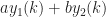
To find answers to these questions, we can conceive of applying an averaging operation, knowing that if the additive noise at each sample is independent of the additive noise at the others, and the additive noise has a mean of zero, then such averaging will tend to suppress the effects of the noise while maintaining the presence of the non-noise component of the signal. If the signal component of the data is itself not independent sample-to-sample, then it will not be averaged away by the averaging process. The output of such an averaging operation is $y(k)$ . We’ll define the value of $y(k)$ to be the arithmetic average of the preceding $N-1$ points of $x(k)$ and $x(k)$ itself:

$\displaystyle y(k) = \frac{1}{N} \sum_{j=k-N+1}^k x(j) \hfill (1)$

This is illustrated in Figure 2.

Figure 2. Illustration of the endpoints of the moving-average filter “window” for time $k$ . Here $y(9) = [x(9) + x(8) + x(7) + x(6) + x(5)]/5$ because $N=5$ .

This averaging operation moves along with time, and so it is understandably called a moving average, as we mentioned at the top of the post.

Is this moving average operation a linear time-invariant system? First, let’s check for linearity. Let $x_1(t) \mapsto y_1(k)$ and $x_2(k) \mapsto y_2(k)$ . Then what is the output for $x(k) = ax_1(k) + bx_2(k)$ ? If the system is linear, it must be $a y_1(k) + b y_2(k)$ . We have the output

$\displaystyle y(k) = \frac{1}{N} \sum_{j=k-N+1}^k x(j) = \frac{1}{N} \sum_{j=k-N+1}^k (ax_1(j) + bx_2(j)) \hfill (2)$

$\displaystyle = \frac{a}{N} \sum_{j=k-N+1}^k x_1(j) + \frac{b}{N} \sum_{j=k-N+1}^k x_2(j) \hfill (3)$

$\displaystyle = a \left(\frac{1}{N} \sum_{j=k-N+1}^k x_1(j) \right) + b \left(\frac{1}{N} \sum_{j=k-N+1}^k x_2(j) \right) \hfill (4)$

$\displaystyle = ay_1(k) + by_2(k). \hfill (5)$

So that the defined moving-average operation is linear.

Next we test for time-invariance (here, in discrete time, this is often called shift invariance). If the system is time invariant, then the output for a shifted version of an input is just the shifted output for the original unshifted input. Let $x(k) \mapsto y(k)$ . Then look at the output for input $x(k-k_0)$ . If this is equal to $y(k-k_0)$ , then the moving-average system is time-invariant. Let’s take a look.

$\displaystyle x(k-k_0) \mapsto y_0(k) = \frac{1}{N} \sum_{j=k-N+1}^k x(j-k_0). \hfill (6)$

Is $y_0(k) = y(k-k_0)$ ? Let’s perform a substitution for $j$ to find the answer. Let $n=j-k_0$ . Then if $j=k-N+1$ , $n= k-k_0 - N + 1$ . Similarly, if $j=k$ , then $n = k-k_0$ . Our output signal $y_0(k)$ becomes

$\displaystyle y_0(k) = \frac{1}{N} \sum_{n=k-k_0-N+1}^{k-k_0} x(n). \hfill (7)$ .

But the right side of (7) is, by definition, $y(k-k_0)$ . So we have

$\displaystyle x(k-k_0) \mapsto y_0(k) = y(k- k_0) \hfill (8)$

and therefore the defined moving-average operation is time-invariant. Since the moving-average operation is equivalent to a linear time-invariant system, it can be represented by an impulse-response function or a frequency-response function (transfer function). Let’s find expressions for each of these key system input-output functions.

Impulse Response Function

To find the impulse-response function, we simply apply an input that is equal to the discrete-time impulse $\delta(k)$ , which is shown in Figure 3, and determine the value of $y(k)$ for each possible $k$ . In this situation, we rename $y(k)$ as $h(k)$ , the conventional symbol used for impulse-response functions in both continuous and discrete time.

Figure 3. The discrete-time impulse function.

$\displaystyle y(k) = \frac{1}{N} \sum_{j=k-N+1}^k x(k), \hfill (9)$

implies that the impulse response is given by

$\displaystyle h(k) = \frac{1}{N} \sum_{j=k-N+1}^k \delta(k). \hfill (10)$

Since $\delta(j)$ is zero except at $j=0$ , where it is equal to 1, $h(k)$ will be zero whenever the summation interval $[k-N+1, k]$ does not contain $j=0$ . Thus, for all $k<0$ , we have the interval $[k-N+1, k]$ which is entirely to the left of zero, provided that $N \ge 1$ (which we assume is true). Therefore, the impulse response is zero for all negative values of $k$ .

When $k=0$ , the summation interval is $[-N+1, 0]$ , which does contain zero at the right edge, and so we have

$\displaystyle h(0) = \frac{1}{N} \sum_{j=-N+1}^0 \delta(j) = 1/N. \hfill (11)$

For $k=1$ , we have

$\displaystyle h(1) = \frac{1}{N} \sum_{j=2-N}^1 \delta(j), \hfill (12)$

which is equal to $1/N$ provided that $N \ge 1$ , as already assumed. This pattern continues, with the value of $h(k)$ being $1/N$ until $k = N-1$ . For $k=N$ , the summation interval is $[1, N]$ , which no longer contains zero, and so $h(N) = 0$ . For $k > N$ , the interval continues to slide to the right of zero, and will never again contain zero, so that $h(k) = 0, k \ge N$ . In summary, we have the impulse-response function

$\displaystyle h(k) = \left\{ \begin{array}{ll} 0, & k < 0, k \ge N \\ 1/N, & 0 \leq k \leq N-1 \end{array} \right. . \hfill (13)$

The impulse-response function for the moving-average filter with length $N$ is simply a rectangle with width $N$ and height $1/N$ . The impulse response is graphed in Figure 4. This is consistent with the intended operation of the filter: sum the previous $N-1$ signal values and the current signal value, and divide by the number of values you summed, which is $N$ .

Figure 4. The impulse-response function for the moving-average filter with parameter $N$ . It is simply a rectangle with height $1/N$ and width $N$ samples.

Frequency Response

The frequency-response function is defined as the response of the system to a sine-wave input, and can be computed, as we’ve shown in a previous post, using the Fourier transform applied to the impulse response.

$\displaystyle H(f) = \sum_{j=-\infty}^\infty h(j) e^{-i 2 \pi f j}. \hfill (14)$

This version of $H(f)$ uses a continuous frequency variable $f$ . It is periodic with period equal to one. Let’s evaluate the transform in (14), then think about discretizing frequency in anticipation of using a computer to analyze the situation in both discrete time and discrete frequency.

$\displaystyle H(f) = \sum_{j=0}^{N-1} (\frac{1}{/N}) e^{-i 2 \pi f j} \hfill (15)$

$\displaystyle = \frac{1}{N} \sum_{j=0}^{N-1} \left( e^{-i 2 \pi f} \right)^j = \frac{1}{N} \sum_{j=0}^{N-1} c^j, \hfill (16)$

where $c = e^{- i 2 \pi f }$ . This last summation is an example of the general geometric series

$\displaystyle S = \sum_{k=0}^{N-1} a^k = \frac{1-a^N}{1-a}. \hfill (17)$

So the frequency response for the moving-average filter is given by

$\displaystyle H(f) = \frac{1}{N} \left( \frac{1-e^{- i 2 \pi f N}}{1 - e^{-i 2 \pi f}} \right) \hfill (18)$

$\displaystyle = \frac{1}{N} \frac{e^{-i\pi f N} \left( e^{i \pi f N} - e^{-i \pi f N} \right)}{e^{-i\pi f} \left(e^{i\pi f} - e^{-i\pi f}\right)} \hfill (19)$

$\displaystyle = \frac{1}{N} e^{-i \pi f (N-1)} \left( \frac{\sin(\pi f N)}{\sin(\pi f)} \right). \hfill (20)$

Notes on the Frequency Response

We make the following observations about the frequency response.

The derived frequency-response function is similar to the Fourier transform of a continuous-time rectangle function, which is a sinc function, but it is not identical to a sinc. In particular, the denominator contains the $\sin(\cdot)$ function instead of being proportional to $f$ .
The derived frequency response is periodic with period $1$ . This periodicity follows from the periodicity of the discrete-time Fourier transform.
For small values of $f$ , $\sin(\pi f) \approx \pi f$ , and so $|H(f)| \approx (1/N) \left| \frac{\sin(\pi f N)}{\pi f} \right| = \left| \frac{\sin(\pi f N)}{\pi f N} \right| = | \mbox{\rm sinc}(fN)|$ . Therefore, the bulk of the energy in $H(f)$ is concentrated near $f=0$ . The moving-average filter passes lower frequencies and attenuates or rejects higher frequencies.
$|H(0)| = 1$ since $\mbox{\rm sinc}(0) = 1$ .
$|H(f)| = 0$ for $f = m/N, m\neq 0$ . For example, $H(1/N) = 0$ , which implies that the moving-average filter output is zero for an input sine wave with frequency $1/N$ . (Can you see this from the time-domain operation of the filter?)

Sampled Frequency Response and Zero-Padding

The frequency response we’ve derived is valid for any $f$ , but it is also periodic with period 1. So the important values of $f$ reside in a single period, say $f \in [0, 1]$ . We can look at $M$ samples of the frequency response by simply substituting into our general formula. Say we want to look at the $M$ frequency values

$\displaystyle f_k = k/M, k = 0, 1, 2, \ldots, M-1, \hfill (21)$

where $M \ge N$ . Then we have the sampled frequency-response function

$\displaystyle H(f_k) = H(k/M) = \frac{1}{N} e^{-i \pi k(N-1)/M} \left( \frac{\sin(\pi k N/M)}{\sin(\pi k/M)} \right) \hfill (22)$

for $k = 0, 1, 2, \ldots, M-1$ . How can we compute this set of values using a transform? We have

$\displaystyle H(k/M) = \sum_{j=-\infty}^\infty h(j) e^{-i 2 \pi k j /M} \hfill (23)$

$\displaystyle = \sum_{j=0}^{N-1} h(j) e^{-i 2 \pi k j /M}. \hfill (24)$

To use the power and efficiency of the FFT, we can extend the sum from $N-1$ to $M-1$ , and simply define the missing values of $h(j)$ to be zero. That is, pad $h(j)$ with $M-N$ zeros and compute

$\displaystyle H(k/M) = \sum_{j=0}^{M-1} h(j) e^{-i 2 \pi k j/ M}. \hfill (25)$

This is called zero-padding, and it allows us to flesh out the details of the shape of the frequency-response function. When we use, say, $M=2N$ , we pad with $N$ zeros, and the effect (not proven here) is that the original values of $H(f)$ are preserved, but a new value is inserted between each pair of them. Later in the post we will provide a plot of $H(f)$ that uses $N=10$ and $M=256$ .

Step Response

Let’s switch gears and go back to the time domain to look at the response of the moving-average filter to a unit-step input. Recall that the discrete-time unit-step function is denoted by $u(k)$ , and is equal to one for $k >= 0$ and zero otherwise. Let’s evaluate the convolution sum to determine the step response.

$\displaystyle y(k) = x(k) \otimes h(k) \hfill (26)$

$\displaystyle = u(k) \otimes h(k) \hfill (27)$

$\displaystyle = \sum_{j=-\infty}^\infty h(k-j) u(j). \hfill (28)$

For $k < 0$ , $h(k-j)$ has no non-zero samples for $j \ge 0$ . That is, $h(k-j)$ and $u(j)$ have no overlap where $u(j)$ is nonzero. Therefore, the step-response $y(k) = 0$ for negative values of $k$ .

For $k \ge 0$ and $k \le N-2$ , the overlap between $h$ and $u$ is partial. We obtain

$\displaystyle y(k) = \sum_{j=0}^k h(k-j)(1), \ \ 0 \leq k \leq N-2 \hfill (29)$

$\displaystyle y(k) = \sum_{j=0}^k (1/N) = (k+1)/N, \ \ 0 \leq k \leq N-2. \hfill (30)$

Finally, when $k \ge N-1$ , the overlap is complete, and we have

$\displaystyle y(k) = \sum_{j=k-N+1}^k h(k-j)(1) = \sum_{j=k-N+1}^k \frac{1}{N} = \frac{1}{N} (k - (k-N+1) + 1) = 1. \hfill (31)$

The step response function is shown in Figure 5.

Figure 5. The response of a moving-average filter ( $N=6$ ) to a unit-step-function input. After the start-up phase of the response, from $k=0$ to $k=5$ , the output is equal to one, which is the average value of the step function for large values of $k$ , as expected.

Figure 5. The response of a moving-average filter ( $N=6$ ) to a unit-step-function input. After the start-up phase of the response, from $k=0$ to $k=5$ , the output is equal to one, which is the average value of the step function for large values of $k$ , as expected.

Interconnection of Multiple MA Filters

Here we look at connecting multiple moving-average filters in series, which means that the equivalent linear time-invariant system has a frequency-response function that is the multiplication of the individual moving-average frequency responses. Assume that we connect $K$ identical moving-average filters, each having parameter $N$ and frequency-response function $H(f)$ . Then the frequency response for the equivalent system is $G(f)$ ,

$\displaystyle G(f) = \prod_{j=1}^K H(f). \hfill (32)$

On the other hand, the impulse response for the equivalent system is the convolution of the $K$ individual impulse-response functions,

$\displaystyle g(k) = h(k) \otimes h(k) \otimes \ldots \otimes h(k). \hfill (33)$

What do the impulse responses and frequency responses look like as a function of $K$ ? We’ve already encountered the idea of convolving a rectangle with itself multiple times, so we know, for example, that for $K=2$ , the function $g(k)$ will be a triangle. More importantly, the frequency response as a function of $K$ becomes more and more selective. That is, the attenuation of input frequency components far away from $f=0$ gets very large as $K$ grows. The impulse and frequency-response functions for various $K$ are shown in Figure 6. In this figure, the frequency responses were calculated by Fourier transforming a zero-padded version of the corresponding impulse responses. In terms of the variables defined above, we have $N=10$ and $M = 256$ . This permits a relatively fine sampling of the frequency-response functions.

Figure 6. The impulse-response and frequency-response functions for $K$ serially connected identical moving-average filters with parameter $N=10$ .

A Look at the Residual of the MA Filter

The moving-average filter output reveals the trends, if any, exhibited by the underlying noise-free data, and so is useful as a way to “de-noise” arbitrary datasets. But it may also be of interest to determine the properties of the noise that is rejected by the filter. In this case we want to find the trends with the moving-average filter, then remove them from the input, leaving only the high-frequency fluctuations and no trending signals to contaminate them.

Mathematically, the signal we desire is the input minus the moving-average output,

$\displaystyle z(k) = x(k) - y(k). \hfill (34)$

This can be expressed as the following function of time

$\displaystyle z(k) = x(k) - \frac{1}{N} \sum_{j=k-N+1}^k x(j) \hfill (35)$

$\displaystyle = x(k) - (1/N)x(k-N+1) -(1/N)x(k-N+2) - \ldots - (1/N)x(k) \hfill (36)$

$\displaystyle = \frac{-1}{N}\sum_{j=k-N+1}^{k-1} + \frac{N-1}{N} x(k), \hfill (37)$

which isn’t particularly revealing. Instead, we can attempt to use previous results and approaches to simplify the analysis. The signal $x(k)$ can be obtained by convolving itself with an impulse, and $y(k)$ is obtained by convolving $x(k)$ with $h(k)$ as in Figure 7.

Figure 7. Equivalent linear time-invariant system for extracting the noisy residual from a moving-average operation.

Since we know $h(k)$ is a rectangle with height $1/N$ and width $N$ , we easily obtain $g(k)$ as in Figure 8.

Figure 8. The impulse response for the linear time-invariant system that produces the noisy residual associated with the moving-average operation, rather than the noise-reduced underlying signal.

The frequency response is

$\displaystyle G(f) = {\cal F} \left[ \delta(k) \right] - H(f) \hfill (38)$

$\displaystyle = 1 - H(f) \hfill (39)$

$\displaystyle = 1 - \frac{1}{N} e^{-i \pi f(N-1)} \left( \frac{\sin(\pi f N)}{\sin(\pi f)} \right). \hfill (40)$

The impulse response $g(k)$ and corresponding frequency response $G(f)$ are plotted in Figure 9. It is clear that this filter passes only relatively high frequencies, providing the desired inverse operation relative to a moving average.

Figure 9. The impulse and frequency response for a residual moving-average filter.

Significance of Moving-Average Filters in CSP

The main use I have for a moving-average filter is as a smoothing filter in the frequency-smoothing method (FSM) of spectral correlation function estimation. Certain kinds of specialized signal-to-noise ratio calculations can also benefit from the use of a fast smoothing operation, and the computational cost of a moving-average filtering operation is quite low because of the unique shape of the impulse response–a rectangle. This enables the use of a head-tail running sum to implement the convolution, avoiding having to do $N$ multiplications for each output point of the filter.

Previous SPTK Post: Ideal Filters Next SPTK Post: The Complex Envelope

Author: Chad Spooner

I'm a signal processing researcher specializing in cyclostationary signal processing (CSP) for communication signals. I hope to use this blog to help others with their cyclo-projects and to learn more about how CSP is being used and extended worldwide. View all posts by Chad Spooner

3 thoughts on “SPTK: The Moving-Average Filter”

Curt says:

October 3, 2023 at 5:02 pm

Great explanation of a MA filter. Does a MA filter incorporate amplitude modulation automatically or is there an additional parameter, such as a constant, that can be used in your filter design?

Loading...

1. Chad Spooner says:
  
  October 4, 2023 at 10:43 am
  
  Welcome to the CSP Blog Curt! Thanks for the comment.
  
  The moving-average filter I examine in the post, with impulse-response function shown in Figure 4, is a true averager in that it preserves amplitude. Because the sum of the elements of the impulse response is one, if you apply the filter to a constant signal, the output is identical to the input. So a constant signal having value of 10 produces a constant signal with a value of 10 at the output. If you want to scale the signal as well as filter away the relatively high-frequency noise, you can definitely scale the impulse response function. But you could also just multiply the output of the filter by the desired constant.
  
  A drawback of scaling the impulse-response function is that the ‘head-tail’ summation trick, mentioned in the final ‘Significance’ section of the post, is not straightforward. In fact, the way I described it is a bit unclear. To use the computationally low-cost ‘head-tail’ summation trick with the moving-average filter, you need to scale the impulse response in Figure 4 so that each non-zero element is equal to one. Then apply the filter, using ‘head-tail’ summation, and finally at the end multiply by 1/N.
  
  Does my response address what you meant by ‘amplitude modulation?’
  
  Loading...
  
  1. Curt Mitchell says:
    
    October 16, 2023 at 11:23 am
    
    Yes it does Chad. It was very clear. Thanks!
    
    Loading...