CSP Estimators: The FFT Accumulation Method

An alternative to the strip spectral correlation analyzer.

Let’s look at another spectral correlation function estimator: the FFT Accumulation Method (FAM). This estimator is in the time-smoothing category, is exhaustive in that it is designed to compute estimates of the spectral correlation function over its entire principal domain, and is efficient, so that it is a competitor to the Strip Spectral Correlation Analyzer (SSCA) method. I implemented my version of the FAM by using the paper by Roberts et al (The Literature [R4]). If you follow the equations closely, you can successfully implement the estimator from that paper. The tricky part, as with the SSCA, is correctly associating the outputs of the coded equations to their proper $\displaystyle (f, \alpha)$ values.

We’ll also implement a coherence computation in our FAM, and use it to automatically detect the significant cycle frequencies, just as we like to do with the SSCA. Finally, we’ll compare outputs between the SSCA and FAM spectral-correlation and spectral-coherence estimation methods. The algorithms’ implementations are not without issues and mysteries, and we’ll point them out too. Please leave corrections, comments, and clarifications in the comment section.

Definition of the FFT Accumulation Method

The method produces a large number of point estimates of the cross spectral correlation function. In [R4], the point estimates are given by

$\displaystyle S_{xy_T}^{\alpha_i + q\Delta\alpha} (rL, f_j)_{\Delta\!t} = \sum_{r}X_T(rL, f_k) Y_T^* (rL, f_l) g_c(n-r) e^{-i2\pi r q /P} \hfill (1)$

where the complex demodulates are given by

$\displaystyle X_T(n,f) = \sum_{r=-N^\prime/2}^{N^\prime/2} a(r) x(n-r) e^{-i 2 \pi f(n-r)T_s} \hfill (2)$

Equation (2) here is Equation (2) in [R4]. I think it should have a sum over $N^\prime$ samples, rather than $N^\prime+1$ ,

$\displaystyle X_T(n,f) = \sum_{r=-N^\prime/2}^{N^\prime/2-1} a(r) x(n-r) e^{-i 2 \pi f(n-r)T_s} \hfill (3)$

In (1), the function $g_c(n)$ is a data-tapering window, which is commonly taken to be a unit-height rectangle (and therefore no actual multiplications are needed), and in (2), the function $a(r)$ is another tapering window, which is often taken to be a Hamming window (can be generated using MATLAB’s hamming.m).

The sampling rate is $\displaystyle f_s = 1/T_s$ . In (2) and (3), $\displaystyle T = N^\prime T_s$ . The channelizer (short-time hopped) Fourier transforms’ tapering window $\displaystyle a(r)$ has width $\displaystyle T_s N^\prime$ , and the output (long-time) Fourier transforms’ tapering window $\displaystyle g_c(r)$ has width $NT_s$ , which is the length of the data-block that is processed.

So the FAM channelizes the input data using short Fourier transforms of length $\displaystyle N^\prime$ , which are hopped in time by $L$ samples. This results in a sequence of transforms that has length

$\displaystyle P = N/L \hfill (4)$

where here I am assuming that both $N$ and $L$ are dyadic integers, with $L \ll N$ . Therefore, the length of the output Fourier transforms is $P$ .

For (1), [R4] defines the cycle-frequency resolution as

$\displaystyle \Delta\alpha = 1/N \hfill (5)$

in normalized-frequency units. Finally, the point estimate is associated with the cycle frequency $\displaystyle \alpha_i$ and the spectral frequency $\displaystyle f_j$ , which are defined in terms of the spectral components involved in the output transform:

$\displaystyle \alpha_i = f_k - f_l \hfill (6)$

and

$\displaystyle f_j = (f_k + f_l)/2 \hfill (7)$

Basic Steps in Implementing the FAM in Software

Step 1: Find and Arrange the $\displaystyle N^\prime$ -Point Data Subblocks

Thinking in terms of MATLAB coding, we’d like to perform as many vector or matrix operations as possible, and as few for-loop operations as possible. So when we extract our blocks of $N^\prime$ samples, sliding along by $L$ samples, we can place each one in a column of a matrix:

fam_data_blocks

Note that to achieve the full set of $P$ blocks, we’ll need to add a few zeroes to the end of the input $x(t)$ . So now we have a matrix with $N^\prime$ rows and $P$ columns.

Step 2: Apply Data-Tapering Window to Subblocks

We will be Fourier transforming each column of the data-block matrix from Step 1, but before that we’ll apply the channelizer data-tapering window called $a(\cdot)$ above. Let’s pick the Hamming window, available in MATLAB as the m-file function hamming.m. Let’s denote this particular choice for $a(\cdot)$ by $h(\cdot)$ . Each column of our data-block matrix needs to be multiplied by a Hamming window with length $N^\prime$ :

fam_data_blocks_window

Step 3: Apply Fourier Transform to Windowed Subblocks

Next, apply the Fourier transform to each column. This is easy in MATLAB with fft.m, but there is a complication. The relative delay that exists between each of the blocks in the matrix is lost when fft.m is applied to each column. That is, (2) above is not exactly computed; the phase relationship between the transforms is modified through the use of fft.m, which we want to use for computational efficiency.

fam_channelized

So after the FFT is applied to the data blocks, they need to be phase-shifted. The phase shift for a particular element depends on the frequency $f_j$ and the time index $rL$ . This is similar to what we do in the time-smoothing method of spectral correlation estimation; see this post for details.

Do the same thing for the input $y(t)$ . If $x(t) == y(t)$ , then don’t bother repeating the computation, otherwise, do so:

fam_channelized_Y

Step 4: Multiply Channelized Subblocks Together and Fourier Transform

Looking back at (1), we now need to multiply (elementwise) one row from the $X$ matrix by one row from the $Y$ matrix, conjugating the latter. This will result in a vector of $P$ complex values, which can then be transformed using the FFT. For example, below I’ve boxed the $X$ values for $f_k = f_1$ and the $Y$ values for $f_l = f_2$ .

fam_channelized_boxed

fam_channels_Y_boxed

Step 5: Associate Each Fourier Transform Output with the Correct $\displaystyle (f, \alpha)$

According to (1), the $P$ values that arise from the Fourier transform of the channelizer product vector correspond to the $P$ cycle frequencies

$\displaystyle \alpha_i + q\Delta \alpha \hfill (8)$

where $\displaystyle \Delta\alpha$ and $\displaystyle \alpha_i$ are defined in (5) and (6), and $q$ ranges over $P$ integers. This association leads to values in the familiar diamond-shaped principal domain of the spectral correlation function; any values that do not lie in that region can be discarded. So at this point, we have a large number of spectral correlation function point estimates for frequencies in the (normalized) range $\displaystyle [-0.5, 0.5)$ and cycle frequencies in the range $\displaystyle [-1.0, 1.0)$ .

Extension to the Conjugate Spectral Correlation Function

If $\displaystyle x(t) = y(t)$ , then $\displaystyle Y_T(t,f) = X_T(t,f)$ , and the estimate produced by (1) corresponds to the (auto) non-conjugate spectral correlation function. If $\displaystyle y(t) = x^*(t)$ , then the estimate corresponds to the conjugate spectral correlation function. Otherwise, it is a generic cross spectral correlation function. The extension to the conjugate spectral correlation function is that easy! It’s only a little more complicated to extend the conjugate spectral correlation function to the conjugate coherence than it is to extend the non-conjugate spectral correlation to the non-conjugate coherence.

Extension to Coherence

Recall that the spectral coherence function, or just coherence, is defined for the non-conjugate spectral correlation function by

$\displaystyle C_x^\alpha(f) = \frac{S_x^\alpha(f)}{\left[ S_x^0(f+\alpha/2)S_x^0(f-\alpha/2) \right]^{1/2}} \hfill (9)$

The conjugate coherence is given by

$\displaystyle C_{x^*}^\alpha(f) = \frac{S_{x^*}^\alpha(f)}{\left[ S_x^0(f+\alpha/2) S_x^0(\alpha/2 - f) \right]^{1/2}} \hfill (10)$

To compute estimates of the coherence, then, go through the spectral correlation estimates one by one, find the associated spectral frequency $f$ and cycle frequency $\alpha$ from Step 5, and then use a PSD estimate to find the corresponding two PSD values that form the normalization factor. I typically use a side estimate of the PSD that is highly oversampled so it is easy to find the required PSD values for any valid combination of spectral frequency $f$ and cycle-frequency shift $\pm\alpha/2$ . The frequency-smoothing method is a good choice for creating such PSD estimates.

The coherence is especially useful for automatic detection of significant cycle frequencies in a way that is invariant to signal and noise power levels, as described in the comments of the SSCA post.

Examples

Let’s look at the output of the FAM I’ve implemented with an eye toward comparing to the strip spectral correlation analyzer and (of course!) to the known spectral correlation surface for our old friend the rectangular-pulse BPSK signal.

Rectangular-Pulse BPSK (Textbook Signal)

First, let’s review the theoretical spectral correlation function for a rectangular-pulse BPSK signal with independent and identically distributed bits, ten samples per bit, and a carrier offset of $0.05$ :

ww_ideal_scf_BPSK_fs_1 — Figure 1. Theoretical spectral correlation surfaces for rectangular-pulse BPSK. These arise from numerical evaluation of the known spectral correlation formula for BPSK.

The signal exhibits non-conjugate cycle frequencies that are multiples of the bit rate, or $\displaystyle \alpha = kf_{bit}, k = 0, \pm 1, \pm 2, \ldots$ , which for $\displaystyle f_{bit} = 0.1$ is the set $\displaystyle \{0, \pm 0.1, \pm 0.2, \ldots\}$ . Due to symmetry considerations, we ignore the negative non-conjugate cycle frequencies in our plots.

It also exhibits the conjugate cycle frequencies that are the non-conjugate cycle frequencies plus the doubled carrier $2f_c = 2(0.05) = 0.1$ . The shape of the conjugate spectral correlation function for $\alpha = 2f_c$ is the same as that for the non-conjugate spectral correlation function for $\alpha = 0$ (the PSD).

Let’s start the progression of FAM results for rectangular-pulse BPSK with the FAM power spectrum estimate together with a TSM-based PSD estimate for comparison:

fam_tsm_psd_plot_bpsk — Figure 2. Comparison of two power spectral density estimates: The FAM and the time-smoothing method (TSM).

Both PSD estimates look like what we expect for the signal, but you can see a small regular ripple in the FAM estimate, which is not in the TSM estimate, and which we know is not a true feature of the PSD for the signal. So that is a mystery I’ve not yet solved. We’ll see, though, that overall the FAM implementation I’ve created compares well to the SSCA outputs in terms of cycle frequencies, spectral correlation magnitudes, and spectral coherence magnitudes.

Next, I want to show the FAM-based non-conjugate and conjugate spectral correlation surfaces. Let’s first mention the processing parameters:

- - $\displaystyle N = 32768$
  - $\displaystyle N^\prime = 32$
  - $\displaystyle L = N^\prime / 4$
  - $\displaystyle P_{FA} = 10^{-9}$

The latter parameter is used, together with $N$ and $N^\prime$ , to compute a threshold for the coherence function. Only those point estimates that correspond to a coherence magnitude that exceeds the threshold are included in the following FAM spectral correlation surface plots:

fam_surf_nonconj_bpsk — Figure 3. FAM-produced non-conjugate spectral correlation function estimates.

fam_surf_conj_bpsk — Figure 4. FAM-produced conjugate spectral correlation function estimates.

So the FAM surfaces agree with the ideal surfaces in terms of the known cycle frequency values and the variation over spectral frequency $f$ for each coherence-detected $\alpha$ . In other words, it works.

In the following graphs, I show the cyclic domain profiles for the FAM and for the SSCA for comparison:

fam_ssca_cdp_scf_nc_bpsk — Figure 5. FAM-produced and SSCA-produced non-conjugate spectral-correlation cyclic-domain profile results for rectangular-pulse BPSK.

fam_ssca_cdp_scf_c_bpsk — Figure 6. FAM-produced and SSCA-produced conjugate spectral-correlation cyclic-domain profile estimates.

fam_ssca_cdp_coh_nc_bpsk — Figure 7. FAM-produced and SSCA-produced non-conjugate spectral-coherence cyclic-domain profile results for rectangular-pulse BPSK.

fam_ssca_cdp_coh_c_bpsk — Figure 8. FAM-produced and SSCA-produced conjugate spectral-coherence cyclic-domain profile results for rectangular-pulse BPSK.

Finally, here are plots of only the coherence-threshold detected cycle frequencies, which is a typical desired output in CSP practice:

fam_ssca_cfs_scf_nc_bpsk — Figure 9. FAM-produced and SSCA-produced non-conjugate spectral-correlation cyclic-domain profile results for rectangular-pulse BPSK showing only those cycle frequencies with coherence magnitudes that cross a threshold.

fam_ssca_cfs_coh_nc_bpsk — Figure 10. FAM-produced and SSCA-produced non-conjugate spectral-coherence cyclic-domain profile results for rectangular-pulse BPSK showing only those cycle frequencies with coherence magnitudes that cross a threshold.

fam_ssca_cfs_scf_c_bpsk — Figure 11. FAM-produced and SSCA-produced conjugate spectral-correlation cyclic-domain profile results for rectangular-pulse BPSK showing only those cycle frequencies with coherence magnitudes that cross a threshold.

fam_ssca_cfs_coh_c_bpsk — Figure 12. FAM-produced and SSCA-produced conjugate spectral-coherence cyclic-domain profile results for rectangular-pulse BPSK showing only those cycle frequencies with coherence magnitudes that cross a threshold.

Only true cycle frequencies are detected by both algorithms. The average values for spectral correlation and coherence for all the other cycle frequencies are about the same between the FAM and the SSCA. Two anomalies are worth mentioning. The first is that the SSCA produces a coherence significantly greater than one for the doubled-carrier conjugate cycle frequency of $0.1$ . The second is that the FAM produces a few false peaks in the spectral correlation function (near $0.6, 0.7,$ and $0.8$ ). These all have coherence magnitudes that do not exceed threshold, so they don’t end up getting detected and don’t appear in the later plots. I don’t yet know the origin of these spurious spectral correlation peaks, and if you have an idea about it, feel free to leave a comment below.

Captured DSSS BPSK

Let’s end this post by showing FAM and SSCA results for a non-textbook signal, a captured DSSS BPSK signal. Recall that DSSS BPSK has many cycle frequencies, both non-conjugate and conjugate, and that the number of cycle frequencies increases as the processing gain increases. See the DSSS post and the SCF Gallery post for more details and examples.

In this example, the sampling rate is arbitrarily set to $5$ MHz, and the number of processed samples is $N = 65536$ .

fam_tsm_psd_plot_dsss — Figure 13. FAM-produced and TSM-produced power spectrum estimates for a captured DSSS BPSK signal.

fam_surf_nonconj_dsss — Figure 14. FAM-produced non-conjugate spectral correlation surface for a captured DSSS BPSK signal.

fam_surf_conj_dsss — Figure 15. FAM-produced conjugate spectral correlation surface for a captured DSSS BPSK signal.

fam_ssca_cdp_scf_nc_dsss — Figure 16. FAM-produced and SSCA-produced non-conjugate spectral correlation cyclic-domain profile for a captured DSSS BPSK signal.

fam_ssca_cdp_scf_c_dsss — Figure 17. FAM-produced and SSCA-produced conjugate spectral correlation cyclic-domain profile for a captured DSSS BPSK signal.

fam_ssca_cdp_coh_nc_dsss — Figure 18. FAM-produced and SSCA-produced non-conjugate spectral coherence cyclic-domain profile for a captured DSSS BPSK signal.

fam_ssca_cdp_coh_c_dsss — Figure 19. FAM-produced and SSCA-produced conjugate spectral coherence cyclic-domain profile for a captured DSSS BPSK signal.

fam_ssca_cfs_scf_nc_dsss — Figure 20. FAM-produced and SSCA-produced non-conjugate spectral correlation cyclic-domain profile for a captured DSSS BPSK signal using only those cycle frequencies that have coherence magnitudes that exceed a threshold.

fam_ssca_cfs_scf_c_dsss — Figure 21. FAM-produced and SSCA-produced conjugate spectral correlation cyclic-domain profile for a captured DSSS BPSK signal using only those cycle frequencies that have coherence magnitudes that exceed a threshold.

fam_ssca_cfs_coh_nc_dsss — Figure 22. FAM-produced and SSCA-produced non-conjugate spectral coherence cyclic-domain profile for a captured DSSS BPSK signal using only those cycle frequencies that have coherence magnitudes that exceed a threshold.

fam_ssca_cfs_coh_c_dsss — Figure 23. FAM-produced and SSCA-produced conjugate spectral coherence cyclic-domain profile for a captured DSSS BPSK signal using only those cycle frequencies that have coherence magnitudes that exceed a threshold.

Support the CSP Blog here.

Author: Chad Spooner

I'm a signal processing researcher specializing in cyclostationary signal processing (CSP) for communication signals. I hope to use this blog to help others with their cyclo-projects and to learn more about how CSP is being used and extended worldwide. View all posts by Chad Spooner

130 thoughts on “CSP Estimators: The FFT Accumulation Method”

Mirko von Leipzig says:

June 11, 2018 at 12:50 am

I’m curious if choosing different window functions would help alleviate the differences between FAM and SSCA. I know that common practice is a window to determine spectral peak location, and a completely different one to accurately determine actual peak power.

A Hann/Hamming window is a middle ground window AFAIK – a bit of both worlds.

Reply
1. Chad Spooner says:
  
  June 11, 2018 at 5:07 pm
  
  That sounds right to me. I actually use a different window on the “channelizer” Fourier transforms in the SSCA than I do in the FAM. I should redo a couple of those FAM/SSCA comparison calculations using a couple different windows–and show a couple where the two algorithms use the same window. Thanks Mirko!
  
  Reply
  1. Riley H says:
    
    December 17, 2021 at 8:45 am
    
    Hey Mr. Spooner, what was the result of matching the widows? Did the ripples go away?
    
    Reply
  2. Riley H says:
    
    December 17, 2021 at 9:29 am
    
    Hey Chad, did you see if changing filters resolved the ripple issue?
    
    Reply
    1. Chad Spooner says:
      
      December 23, 2021 at 3:40 pm
      
      Thanks for visiting the CSP Blog Riley!
      
      Filters or tapering windows do not seem to be the problem. I can force the output of the FAM to be highly consistent with theory (the non-conjugate and conjugate SCF estimates match theoretical formulas) if I decimate the frequency vector by a factor of two. So there is some kind of stray oscillation associated with a factor of $e^{i\pi k}$ or the like in my code. Presumably my code matches the formulas in the post, in which case something is subtly off in those formulas, but it doesn’t stop the FAM, as presented, from being just as useful as the SSCA.
      
      Here are two results where I simply plot the PSD or the SCF against the frequency vector as I’ve defined it in the post:
      
      And here are the same estimates, but I’m only plotting every other frequency:
      
      Reply
      1. Riley H says:
        
        January 3, 2022 at 11:44 am
        
        Interesting, I am having similar ripples and have an idea of where they come from. I cant speak for your code, but in mine the ripples come from trying to map f_j into integers to store into a matrix. If you want spots for all the cycle frequencies, then for the PSD (a_i = 0) there must be zeros in between each f_j so there is a spot to place the value for the next a_(i+1) that corresponds to the correct f_j. Thus if you decimate the problem goes away. I hope that makes sense, I would be very interested to see if there is something similar going on in you implementation.
        
        Thanks for the blog,
        Riley
      2. Chad Spooner says:
        
        January 7, 2022 at 9:30 am
        
        Well, the rippling I observe does not involve zeros. The points I discard are simply slightly attenuated relative to the points I retain.
        
        I have to get to the bottom of this!
      3. Dan Poppert says:
        
        July 26, 2022 at 2:05 pm
        
        Dr. Spooner,
        
        First off thank you for putting together this very informative and useful blog.
        
        Regarding the ripple that you are seeing at the output of the FAM, this may be the natural result of the variable frequency resolution of the FAM, which seems like one disadvantage of this technique over the SSCM. I believe this would have the symptoms you describe here, as dropping every other bin would result in a smoother output. This is because every other bin has the same frequency resolution for a particular cycle frequency, but immediately adjacent bins do not. If I’m correct about the problem you are seeing, combining adjacent estimates in the spectral frequency dimension for the same cycle frequency can help alleviate this problem as this results in a constant frequency resolution.
        
        -Dan
      4. Chad Spooner says:
        
        July 29, 2022 at 3:33 am
        
        Thanks for the compliment, Dan, and for the comment! Much appreciated.
        
        I think you are right. Reader Jonas has also pointed this out.
        
        Please feel free to elaborate with equations or graphs on further comments if you’d like. You can’t directly add images to comments using WordPress.com (my host), but if you send me the images I can integrate them with any comment you leave. Just a thought. “The CSP Blog–Now with Crowdsourcing!”
ÖZKAN AKBUNAR says:

August 8, 2018 at 3:50 am

Hi Mr.Spooner
I couldnt understand how shift phase of data after fft in step (3), it is also not clear in time smoothing post for me. I will be appreciated if you will explain what is it ?

Best regards.

Reply
1. Chad Spooner says:
  
  August 8, 2018 at 3:19 pm
  
  Looking at Eq (1) in the TSM post, we see that the right side is almost the DFT (FFT). The difference is in the argument of the data function $x(\cdot)$ , which is $t+u$ . If $u=0$ , the right side is the DFT. So as we slide along in time with $u$ , the increasing value of $u$ causes the appearance of a complex exponential factor multiplying a DFT. When we use the FFT to compute the DFT, this factor is ignored because each call to the FFT function processes a data vector that starts at time equal to zero.
  
  In other words, take (1) and evaluate (write the equation) it for $u=0$ and for $u= N$ . You will see that the latter possesses the same form as the former, but also has a complex exponential factor.
  
  If we use the FFT to compute the transforms of successive blocks, we’ll lose the phase relationship between the frequency components for some $f$ in each block. So we have to compensate for that. The $X(u, f+\alpha/2)$ factor in the cyclic periodogram is shifted by $e^{i 2 \pi (f + \alpha/2)u}$ and the factor $X(u, f-\alpha/2)$ is shifted by $e^{-i2\pi(f-\alpha/2)u}$ . These multiply to yield a factor of $e^{i 2 \pi \alpha u}$ . Since $u$ takes on the values $1, N, 2N, \ldots, JN, \ldots$ , we need to compensate the $j$ th cyclic periodogram by $e^{-i 2 \pi \alpha j N}$ .
  
  I may have got some minus signs wrong, but that is the basic idea. The FFT is not a sliding transform.
  
  Does that help?
  
  Reply
  1. ÖZKAN AKBUNAR says:
    
    August 15, 2018 at 12:11 am
    
    Thanks Mr.Spooner
    
    I have some questions again, what should be dimensions of matrix which is result of step 4, actually i cant understand how multiply X(rL,f) and its conjugate. You said elementwise multiplication, but I couldnt catch how to multiply elementwise. For instance, should I multiply first rows of two matrix (then second rows and so on), or else?
    In step 5 mapping to cycle frequency and frequency doesnt clear for me, can i do this mapping as SSCA method or i should use different mapping way?
    
    Reply
    1. Chad Spooner says:
      
      August 15, 2018 at 5:59 am
      
      If you want to store the result of Step 4 in a matrix, it would have dimension $(N^\prime)^2 x P$ . Each of the two matrices has $N^\prime$ rows, and you want to multiply all possible pairs of rows. By ‘elementwise multiplication’ I just mean the following. Let $X=[x_1 \ x_2\ x_3]$ and $Y=[y_1\ y_2\ y_3]$ . Then the elementwise multiplication of $X$ and $Y$ is $[x_1y_1\ x_2y_2\ x_3y_3]$ .
      
      The mapping in Step 5 is given by Equations (5), (6), and (8). What is your specific question about that?
      
      Reply
      1. Özkan Akbunar says:
        
        August 17, 2018 at 10:59 am
        
        I understood that formulae but actually I dont understand how i can implement formulae on my matrix in Matlab. This part is not clear for me contrary to first 4 step. Could you explain this part clearly again?
        
        Also, i found some Matlab codes about this topic and i saw that some peoples takes transpose of matrix which is result of step 4 , is it right?
        
        Best regards Mr. Spooner
      2. Chad Spooner says:
        
        August 19, 2018 at 12:24 pm
        
        I am struggling to understand what you don’t understand. Not enough detail in your question?
        
        Regarding your question about some found MATLAB code, I can’t comment on what I can’t see. There are lots of ways to implement an equation, typically, so I can’t say if what you found is correct or not. Does it produce the correct result?
Yorgo Giannakis says:

September 3, 2018 at 3:17 am

Hello Mr. Spooner,
I couldn’t understand how to implement shifted SCFs in Matlab or another simulation environment. For example, let say that alpha and f are equal to 1 an 0.5 respectively. In this situation, f+alpha/2 becomes 1 which is not a value f can take. If f+(or -)alpha/2 exceeds limited region of frequency [-0.5, 0.5), what is the thing I must do?
Thank for valuable contribution to cyclo-lover society.

Reply
1. Chad Spooner says:
  
  September 4, 2018 at 8:48 am
  
  Thanks Yorgo!
  
  Well, the principal domain of the spectral correlation function is a diamond in the $f-\alpha$ plane, and the tips of the diamond are at $(f, \alpha) = (0, \pm 1)$ . But as you note, if you shift the DFT to the left by $\alpha/2 = 0.5$ and to the right by $\alpha/2 = 0.5$ , you will not have any overlap between the two DFTs when you go to multiply them together. So $\alpha = 1$ is a boundary case of little practical importance.
  
  In general, only use those pairs of frequencies $f \pm \alpha/2$ for which each frequency lies in $[-0.5, 0.5)$ , and ignore the rest.
  
  Reply
Yorgo Giannakis says:

September 6, 2018 at 6:40 am

Thanks for your response. I have a new question why we expect the cyclic frequencies at alpha=k*f_bit for integer values of k. I feel that if the PSD is multiplied by PSD shifted with alpha, this multiplication gives a information about SCF. The point I’m wondering is that the PSD is a continuous function of BPSK sign, so why does not the shift of this signal for any alpha value give a peak?

Reply
1. Chad Spooner says:
  
  September 6, 2018 at 7:06 am
  
  The spectral correlation function is not the result of correlating shifted PSDs. It is the correlation between two complex-valued narrowband downconverted components of the input signal. These two narrowband signal components are correlated only when the separation between their center frequencies (before downconversion of course) is equal to a cycle frequency, and the particular cycle frequencies depend on the details of the modulation type of the signal in the input data. Maybe take another look at the introductory post on spectral correlation?
  
  Reply
Manuel Da Costa says:

September 20, 2018 at 1:23 am

Hello Mr. Spooner,
I have some questions about FFT Accumulation Method, firstly, I implemented this method in Matlab to investigate cyclostationary of some basic signal, However, i am stucked at some point, first of all i understood parameter N’ depends on us, or application. I tried my code for different N’ values and I saw a liitle bit different results. What is reason for this and what is optimal way to choose N’ ?
Secondly, sample size of input data is affects cyclic spectrum of signals importantly, is there any way to compansate effects of lower sample sizes?
As you know Matlab is very slow program and computational complexity of algorithm is high.
Thirds, ı investigate cyclic spectrum of OFDM signals especially and i read ur paper which is called “On the Cyclostationarity of OFDM and SC-Linearly Digitally Modulated Signals in Time Dispersive Chnnels: Theoretical Developments and Applications”, but algebra in paper is little bit complex and confusing for me. Can you suggest any resource to understand cyclostationary of OFDM Signals?
Lastly,I am thankful to you for this blog, it really helps me for my workings.
Best regards.
Manuel

Reply
1. Chad Spooner says:
  
  September 20, 2018 at 12:16 pm
  
  Manuel, thanks very much for checking out the CSP Blog. I appreciate readers like you.
  
  Regarding $N^\prime$ , in the FAM it controls the effective spectral resolution $\Delta f$ of the measurement. The total amount of processed data is $N$ samples, which we often call $\Delta t$ . Recall from the post on the resolution product that the variability in an SCF estimate is inversely proportional to the resolution product $\Delta t \Delta f$ .
  
  We know the estimate should get better the larger $N$ is, and for very small $N$ you won’t even be processing a single period of cyclostationarity (for BPSK, the symbol interval), so small $N$ must result in poor estimates. For $N$ larger than that, but still small, I know of little that can be done except through making $\Delta f$ larger.
  
  MATLAB isn’t all that slow in my opinion. It really does not like to do ‘for loops’ though, and nested for loops can definitely slow it down. Try to restructure your MATLAB code so that you eliminate as many for loops as possible (use matrix operations). My FAM implementation takes about 10 seconds to compute the full non-conjugate SCF and coherence for $N= 65536$ , $N^\prime = 32$ , and $L = 8$ . And that includes making several plots.
  
  For the cyclostationarity of OFDM signals, I can only suggest that Google is your friend.
  
  Reply
Manuel Da Costa says:

September 24, 2018 at 1:32 pm

Hello Mr.Spooner
Thanks for your reply, i also read your blog about higher order cyclostationary to calculate cyclic cumulant of any kind of signal but i couldnt imagine how to write code to find cyclic cumulants in Matlab. You said that cyclic cumulant is Fourier series coefficient of higher order cumulant. I thought that if i can calculate higher order cumulant of signal then also find Fourier series coefficients of that cumulant, i can get my cyclic cumulant values. However , I cant find any way how to take values of delay vector in cumulant formula. I took delay vector is zero vector and in that case my cumulant result is scalar and i didnt find Fourier series coefficients. If this idea is true, how i should identify delay vector ?
Secondly, I implemented FAM method as i said in previous comment. I thought, i find cyclic autocorrelation which is second order cyclic cumulant using FAM method, then i also find higher order cyclic cumulunt with this method. Is this idea is true? If this is true how, can you give detailed explanation as in your post FFT Accumulation Method for cyclic autocorrelation and spectral correlation function.
Thank you.
Best Regards.
Manuel

Reply
1. Chad Spooner says:
  
  September 25, 2018 at 9:46 am
  
  i also read your blog about higher order cyclostationary to calculate cyclic cumulant of any kind of signal but i couldnt imagine how to write code to find cyclic cumulants in Matlab. You said that cyclic cumulant is Fourier series coefficient of higher order cumulant. I thought that if i can calculate higher order cumulant of signal then also find Fourier series coefficients of that cumulant, i can get my cyclic cumulant values. However , I cant find any way how to take values of delay vector in cumulant formula. I took delay vector is zero vector and in that case my cumulant result is scalar and i didnt find Fourier series coefficients.
  
  Do you mean the post on moment and cumulant estimators? I think that is a good place for you to start. There are several types of estimators described there, including one that actually produces the time-varying cyclic cumulant function (using synchronized averaging). The delays in the expressions for temporal moments and cumulants are just the delays applied to the input data block before creating a lag product (sometimes called a delay product) such as $L_x(t, \tau_1, \tau_2) = x(t+\tau_1) x^*(t+\tau_2)$ . So you can see that $L_x(\cdot)$ is a function of time (not a scalar), as well as a function of the delays (lags) $\tau_j$ . If the delays are small relative to the block length (a common case), then you can use MATLAB’s circshift.m to implement them with some small loss of fidelity because it is a circular shift rather than a true delay.
  
  If this idea is true, how i should identify delay vector ?
  
  The delay vector choice is driven by the form of the theoretical cyclic cumulant for the signal of interest as well as by the algorithm: what are you going to do with the cyclic cumulant estimates. For many signals, the delay consisting of all zeros corresponds to the cyclic cumulant with the largest magnitude over all possible delay vectors.
  
  Secondly, I implemented FAM method as i said in previous comment. I thought, i find cyclic autocorrelation which is second order cyclic cumulant using FAM method, then i also find higher order cyclic cumulunt with this method. Is this idea is true?
  
  Well, the FAM produces an estimate of the spectral correlation function, which is not the second-order cyclic cumulant. I suppose you could try to inverse Fourier transform the FAM output to get the cyclic autocorrelation, which is indeed the second-order cyclic cumulant for signals that do not contain finite-strength additive sine-wave components. It is difficult to directly use the FAM or SSCA to find the higher order cyclic cumulants. Probably it is best to start in the time domain instead of trying to use the frequency-domain FAM.
  
  If this is true how, can you give detailed explanation as in your post FFT Accumulation Method for cyclic autocorrelation and spectral correlation function.
  
  I think the best thing for you to do is study the post on estimation of higher-order temporal moments and cumulants. Let me know what you think!
  
  Reply
Kevin Young says:

October 10, 2018 at 7:26 pm

Hi Chad
Thank you for your very useful blog!
Here, I have a couple of questions on the implementation of FAM.
1. I understand that after the first N’-point FFT on the windowed signal (step 3), each row denotes a frequency bin from -fs/2:fs/N’:fs/2-fs/N’. After the second P-point FFT on the multiplication of channelized subblocks (step 4), what does each column correspond to?
2. After step 4, I have an array with P x N’ x N’ data. shall I just choose those that satisfies -fs<=alpha<=fs and -0.5*fs<=f<=0.5*fs from P x N' x N' data to generate f-alpha plot?
3. In some thesis (www.dtic.mil/docs/citations/ADA311555), I saw that the author only used P/4:3*P/4 column data (use fft and fftshift) after step 4 to generate f-alpha plot. Do you think it is just for the data filtering purpose?

Reply
1. Chad Spooner says:
  
  October 15, 2018 at 9:28 am
  
  Thanks for your interest and the comment Kevin; I really appreciate readers like you.
  
  1. I understand that after the first N’-point FFT on the windowed signal (step 3), each row denotes a frequency bin from -fs/2:fs/N’:fs/2-fs/N’. After the second P-point FFT on the multiplication of channelized subblocks (step 4), what does each column correspond to?
  
  Do you mean other than Eq (8) in the post? I’m wondering if I’ve been clear in Step 5, which tries to explain the meaning of the various values coming out of the $P$ -point transforms…
  
  2. After step 4, I have an array with P x N’ x N’ data. shall I just choose those that satisfies -fs<=alpha<=fs and -0.5*fs<=f<=0.5*fs from P x N' x N' data to generate f-alpha plot?
  
  Yes, that’s exactly what I do to produce the various plots that I display in the post.
  
  3. In some thesis (www.dtic.mil/docs/citations/ADA311555), I saw that the author only used P/4:3*P/4 column data (use fft and fftshift) after step 4 to generate f-alpha plot. Do you think it is just for the data filtering purpose?
  
  I’m not exactly sure why they chose to do it that way, but I suppose if you carefully do the step above (your question 2, my algorithm Step 5), and keep track of which parts of the $P$ -point transforms you are saving, you might then translate that result into a more efficient step involving the matrix manipulations you mention. I admit that my MATLAB FAM implementation is not optimized for run time; I just wanted to make sure it was essentially correct. I generally use the SSCA for actual CSP work. Good question! Let me know through a comment here if you discover the exact reason why they do what they do in that thesis, and if you agree with it in the end.
  
  Reply
  1. Kevin says:
    
    October 18, 2018 at 7:33 pm
    
    Hi Chad
    
    Thank you for your reply!
    
    On your following comment, I believe your description of Step 5 is clear to me except for the range of q value in equation (8). Is it from -P/2 to P/2-1 or from 0 to P-1?
    
    Do you mean other than Eq (8) in the post? I’m wondering if I’ve been clear in Step 5, which tries to explain the meaning of the various values coming out of the P-point transforms…
    
    Another question I have is when my signal is composed of two different signals, e.g., one sin and one cos function, is the SCF the sum of SCF of sin and cos?
    
    Thanks!
    Kevin
    
    Reply
    1. Chad Spooner says:
      
      October 19, 2018 at 9:52 am
      
      On your following comment, I believe your description of Step 5 is clear to me except for the range of q value in equation (8). Is it from -P/2 to P/2-1 or from 0 to P-1?
      
      Well, did you try each way and see whether one gives the expected answer for an input for which you know the correct set of cycle frequencies and spectral correlation function magnitudes? I start from 0, but this question is probably easily answered by you if you’ve got the basic FAM working.
      
      Another question I have is when my signal is composed of two different signals, e.g., one sin and one cos function, is the SCF the sum of SCF of sin and cos?
      
      This isn’t a completely clear question to me, but it lies in a subtle area of CSP. When you have the sum of statistically independent zero-mean signals, the SCF of the sum is the sum of the SCFs for each summand in the sum. But every word there is important, and “zero-mean” refers to a mean of zero in the fraction-of-time probability framework. That is, a sine wave is not a zero-mean signal in the FOT framework. But if by “sin and cos” you really mean two modulated sine waves in quadrature (such as in QPSK), then, yes, you can add the SCFs for each of the quadrature components provided the modulating signals are themselves statistically independent (which is generally true for QPSK).
      
      For discussions of these kinds of subtle issues, I suggest my two-part HOCS paper (My Papers [5,6]) or my doctoral dissertation.
      
      Reply
  2. Mike says:
    
    September 9, 2021 at 4:30 am
    
    Regarding Kevin Young’s question 3 above, the master’s thesis he mentions is from 1996. An earlier one from 1992 by LCDR Nancy Carter, “Implementation of Cyclic Spectral Analysis Methods,” says this on page 10:
    
    “The product from the previous multiplication is FFT’d to yield a P-point result. Only the middle of the resulting spectrum is retained and stored into the designated f, alpha cell. The upper and lower ends are undesireable because of increased estimate variation at the channel pair ends [Ref. 5:pg 45].”
    
    Carter’s Ref. 5 is Chad’s [R4] by Roberts, Brown and Loomis, and her comment above seems to refer Eqn 32 in the Roberts et al. paper. I also see on Carter’s thesis security form that ‘Name of Responsible Individual’ (her advisor, I assume) is Loomis!
    
    Reply
Taymaz says:

October 28, 2018 at 10:43 pm

Hi Dear spooner,
I am working on an FFT algorithm for acquisition and tracking on weak and high dynamic signals in deep space , can you give me some idea?

Reply
1. Chad Spooner says:
  
  October 30, 2018 at 9:38 am
  
  Taymaz:
  
  Thanks for visiting the CSP Blog.
  
  Can you elaborate on your request? For example, I can’t tell if your problem involves CSP or not. The signal that you might be tracking could be a simple time-varying sine wave, in which case CSP doesn’t have much to offer over Fourier analysis.
  
  Reply
Kevin says:

November 18, 2018 at 7:44 pm

Hi Chad

On the extension to the conjugate spectral correlation function, you explained it based on the auto spectral correlation function. For the cross spectral correlation function x(t)!=y(t), is the conjugate spectral correlation function also calculated by input x(t) and conj(y(t)) using FAM?

Thanks!
K

Reply
1. Chad Spooner says:
  
  November 19, 2018 at 10:27 am
  
  Yes. Suppose we have two time-series $d_1(t)$ and $d_2(t)$ . Then:
  
  If $x(t) = d_1(t)$ and $y(t) = d_1(t)$ , the FAM produces the non-conjugate auto SCF for $d_1(t)$ ,
  if $x(t) = d_1(t)$ and $y(t) = d_1^*(t)$ , the FAM produces the conjugate auto SCF for $d_1(t)$ ,
  if $x(t) = d_1(t)$ and $y(t) = d_2(t)$ , the FAM produces the non-conjugate cross SCF,
  if $x(t) = d_1(t)$ and $y(t) = d_2^*(t)$ , the FAM produces the conjugate cross SCF.
  
  There are two cross versions for each choice of conjugation. That is, you can have $S_{xy}^\alpha(f)$ or $S_{yx}^\alpha(f)$ .
  
  Reply
  1. Kevin says:
    
    November 28, 2018 at 6:42 pm
    
    Hi Chad
    
    When d1(t) and d2(t) are both real signals, non-conjugate SCF should be the same as conjugate SCF. Does it mean we only need to consider non-conjugate/conjugate SCF for complex signals?
    
    Thanks!
    K
    
    Reply
    1. Chad Spooner says:
      
      November 29, 2018 at 6:12 am
      
      Yes. See the post on conjugation configurations for the general $n$ th-order case.
      
      Reply
      1. Kevin says:
        
        November 29, 2018 at 9:06 am
        
        In your rectangular pulse BPSK example, your non-conjugate SCF is different from conjugate SCF. Did you use complex BPSK signal?
        
        Thanks!
        K
      2. Chad Spooner says:
        
        November 29, 2018 at 9:11 am
        
        Yes, see the post on creating a rectangular-pulse BPSK signal. The baseband PAM signal is real-valued for BPSK, but adding the frequency shift by multiplying by a complex-valued exponential renders the signal complex-valued.
Kevin says:

November 29, 2018 at 11:01 am

Got it. You actually used a frequency shifted BPSK rather than a baseband BPSK in this example.

BTW, do you have any blogs on the FRESH filters?

Thanks!
K

Reply
1. Chad Spooner says:
  
  November 29, 2018 at 11:36 am
  
  No, no posts on FRESH filters yet. It is on my to-do list though!
  
  Reply
  1. Kevin says:
    
    December 5, 2018 at 9:13 am
    
    Look forward to your post on FRESH filter.
    
    Here I have one question on this topic. For real signal, we get the same cyclic frequencies for non-conjugate and conjugate SCF. In FRESH filter, do I still need both the linear and conjugate linear branches? Or, shall I just keep the linear branch?
    
    Thanks!
    K
    
    Reply
    1. Chad Spooner says:
      
      December 11, 2018 at 4:19 pm
      
      Just keep the linear branches.
      
      Reply
Kevin Burke says:

February 28, 2019 at 7:55 am

Hi Chad,
A minor typo: comparing (28) in [R4] to equation (1) above suggests there is a missing “equals” sign.
Thanks, Kevin (A different one than the other posts)

Reply
1. Chad Spooner says:
  
  February 28, 2019 at 8:38 am
  
  Kevin Burke:
  
  Thanks for checking out the CSP Blog and taking the time to point out that typo! I really appreciate it. Please don’t hesistate to point out any others, here or via email. cmspooner at ieee dot org.
  
  Reply
Sunson211 says:

March 10, 2019 at 6:03 pm

Dear chad,

Very nice tutorial here. Allow me to have a question here for normalization of SCF by using the equ 9 in the article. By using the example you first figure plot in this article, f is [-0.5 0.5]. Alpha is [0 0.7], Let’s assume I want to calucate the normalized scf button point (f= -0.5 , alpha = 0.7) by using equ 9. But the in the denominator, f – alpha/2 = -0.5 -0.35 = 0.85 !! Which is outside of range of f, right? The f is only between +-0.5 . So, could you advise me ? I think there is something I missed. Thank you so much for your time and help.

Reply
1. Sunson211 says:
  
  March 11, 2019 at 8:23 am
  
  I saw sameone here asked the same question, and your reply is “In general, only use those pairs of frequencies f \pm \alpha/2 for which each frequency lies in [-0.5, 0.5), and ignore the rest.” if my understanding is right, are you saying, i only need to calculate the area if f +- alpha/2 are in [-0.5 0.5]? Could you advise me if I am wrong? Thanks
  
  Reply
  1. Chad Spooner says:
    
    March 11, 2019 at 9:21 am
    
    Yes, that’s right. The “principal domain” for the discrete-time/discrete-frequency spectral correlation function is a diamond with vertices $(f, \alpha) = \{ (-0.5, 0), (0, 1.0), (0.5, 0), (0, -1.0) \}$ . Every point outside of that diamond is redundant with a point inside. Notice that that two-dimensional principal domain contains the normal DSP principal domain of $[-0.5, 0.5]$ .
    
    In your example of one comment back, you chose $(f, \alpha) = (-0.5, 0.7)$ , which is not in the principal domain. So you ended up trying to find the coherence denominator PSD values for frequencies that lie outside of the principal domain for frequencies $[-0.5, 0.5]$ .
    
    Reply
    1. sunson211 says:
      
      March 11, 2019 at 9:59 am
      
      thank you so much for your help! It’s so helpful!!
      Chad, I have few following questions,
      
      1. The normalized SCF (equ 9) plot will be almost the same as original SCF (nominator of equ 9)? What I have now is really different. I got a simple 4QAM baseband orignal SCF, it looks like a peak in the middle of plot. After I did the normalization, I got 4 peaks near 4 corners of plot.
      please check the photo link. this is my first time sharing photo, let let me know it works or not.
      https://photos.app.goo.gl/sTdzwcq4QJbm5wUCA
      
      What i did in the code is,
      1. check the f +- alpha/2 are in the range of [-0.5 0.5] or not. If no, the current scf_norm = 0.
      2. if step 1 is no, then I just find out the current complex value of original scf (equ 9 nominator), then divided by the real number of denominator of equ 9 (the denominator is real number).
      3. then I do abs(equ 9), plot.
      
      Do you think my understanding is correct ? Thank you. Chad.
      
      Reply
      1. Chad Spooner says:
        
        March 11, 2019 at 1:29 pm
        
        The posting of the images to Google Photos worked; I am able to see them.
        
        I don’t see any errors or problems with what you’ve written in your latest comment. However, can you tell me the noise power and the signal power that you used to generate your 4QAM signal? Or, even better, send me the data at cmspooner at ieee dot org.
      2. Chen says:
        
        August 27, 2019 at 7:05 pm
        
        Could you please send the data and code to me?
    2. sunson211 says:
      
      March 11, 2019 at 2:02 pm
      
      Dear Chad,
      
      Thank you again for your help. I will send the data and code to your ieee emai. Thank you again.!
      
      Reply
      1. Minhhuy Le says:
        
        March 28, 2019 at 5:52 pm
        
        Could you please send the data and code to me also
Chinmay Hegde says:

March 12, 2019 at 9:33 am

Hello Dr. Spooner, thanks for the excellent blog. I had a question with regards to your comment about using a side PSD estimate that is highly oversampled in estimating the Coherence functions in (9) and (10). I interpreted that comment to mean that there is a very high sample rate channel for estimating the PSD and a lower sample rate channel for SCF estimation. Is this correct? If not then are you estimating a “finer resolution” PSD via zero-padding or some other form of interpolation? Thanks again!

Reply
1. Chad Spooner says:
  
  March 12, 2019 at 4:32 pm
  
  Thanks for stopping by, Chinmay.
  
  I believe you can take the PSD estimate part of the FAM or SSCA output and interpolate it to create the highly oversampled PSD you need for the coherence calculation. But I typically estimate the PSD on the side, using the TSM or FSM. That gives me lots of control over the resolution and the amount of data that I want to use to make the estimate.
  
  I don’t need two channels–one very high rate and one low–it is just that the resolution of the FAM or SSCA PSD is very coarse. So the original-rate data sequence is just fine.
  
  Reply
  1. Chinmay Hegde says:
    
    March 12, 2019 at 6:52 pm
    
    Ah, ok that is what I did, although I didn’t interpolate the PSD portion of the FAM output. It worked, but I think this might be because I was grossly oversampled to begin with (simulated baseband sample rates of 80-200 MHz compared to baseband signal bandwidths on order of 5-20 MHz).
    
    I also tried computing coherence via a TSM and FSM estimate of the PSD with “finer resolution”, but this introduced more noise into the PSD estimate relative to the PSD portion of the FAM output which in turn resulted in coherence values that could be slightly > 1. (I was working with SNR of 0 dB). In general I didn’t always get coherence values that were 1?
    
    I never ran into the issue of coherence values > 1 when using the TSM or FSM methods (I basically looped over cycle-freqs that I wanted to check when using these methods). Although, in my TSM/FSM implementations I used complex phase shifts in the time domain prior to taking an FFT to compute the +/- alpha/2 freq. shifts required by the cyclic periodogram. As a result, I was taking 2 FFT’s per cycle-freq when computing the non-conjugate SCF via TSM/FSM which gave me “exact” PSD estimates every time I needed them. I was ok with computational burden since I just wanted something to double check my implementation of the FAM method. So far, everything is in agreement outside of the coherence values sometimes being > 1 in my FAM method. (I suspect this is user error on my part).
    
    Thanks again for your reply. And no worries if you are too busy to respond to my most recent queries, your blog has already saved me a lot of time as I try to wrap my head around this stuff.
    
    Reply
Chinmay Hegde says:

March 12, 2019 at 6:58 pm

Sorry, my previous post ended up getting screwed up when I posted. I meant to ask if it makes sense that one might get coherence values > 1 using the FAM method and a side estimate of PSD. I got coherence to be bounded by 1 when using the PSD portion of the FAM SCF but even then it depended on what freq resolution I used (0.5 MHz with 2^15 samples at 200 MHz worked perfectly, but other parameters still sometimes resulted in cohernce slightly > 1). The reason it was confusing to me was that it never happened using my TSM/FSM implementations as described above.

Again, my comment about your relative business with regards to being able to answer still stands 🙂 Thanks!

Reply
1. Chad Spooner says:
  
  March 13, 2019 at 10:10 am
  
  I also get coherence magnitudes greater than 1 sometimes, with both the SSCA and the FAM. I think the reason is almost always that the PSD values used in the normalization of the estimated SCF are poorly resolved. That is, no non-parametric spectrum estimator (such as the TSM, FSM, SSCA, and FAM algorithms, focusing on $\alpha=0$ ) can adequately resolve certain kinds of spectra, such as those containing unit-step-function-like features or impulses. Moreover, when the input data contains little or no noise (as is possible in the world of simulated signals), the spectrum estimators are trying to estimate zero values, so the coherence quotient becomes ill conditioned. Finally, unlike the case of using the TSM or FSM and then computing the coherence, it is difficult to match the spectral resolution of the SSCA or FAM output with the spectral resolution of the side estimate.
  
  So in the end, the coherence quotient will sometimes be poorly estimated, and if the denominator PSD estimates are under estimated, then we’ll get too large of a coherence value relative to theory.
  
  Like spectrum analysis, CSP is a bit of an art, and a bit of a science.
  
  Comments?
  
  Reply
  1. Chinmay Hegde says:
    
    March 13, 2019 at 12:40 pm
    
    Ah, that is a huge relief to hear! I was convinced I must have done something wrong. Yeah everything you said makes sense to me.
    
    Reply
    1. sunson211 says:
      
      March 15, 2019 at 9:59 am
      
      Hi Dr Hegde,
      
      May I have a quick question for you? I am working on this equ 9 for normalization SCF as well. But I got something I dont understand.
      Please check the plot here.
      https://photos.app.goo.gl/LiiT2tQtQNVjBS1x7
      
      the top one is just original SCF, the button one is the normalized one by using equ 9. However, as you seen, it really looks different from original one. I think this must be wrong. Could you give me some hints which could case this problem ? Btw. acutally, I may get value > 1 for normalized SCF, but I just make it = 0 right now….. Thanks.
      
      Reply
      1. Chinmay Hegde says:
        
        March 15, 2019 at 11:12 am
        
        Hello sunson,
        
        Unfortunately I don’t think I can help you by looking at those images. Sorry.
        
        Btw, I actually don’t have a PhD so I’m just Mr. Hegde. Good luck with your work.
        
        -Chinmay
MS says:

April 17, 2019 at 9:48 am

Hi Chad,

Thank you for the interesting post. I have a comment and a question.

The comment is when I used a low value of N’ (say, 16), I get a coherence magnitude that is much greater than 1. Upon inspection, I see that the features from the FAM method is more smeared out than the features for the generated PSD, which I have tried using both the FSM and TSM methods. Due to the smearing, the coherence magnitude is much higher than 1 at these points. When I used N’ = 64, the features from the FAM method match the PSD better and the coherence magnitude is much better. Perhaps the poor resolution of the FAM can lead to erroneous coherence magnitudes.

For the question, what is PFa and how is it used to calculate the threshold for the coherence?

Thank you.

Reply
1. Chad Spooner says:
  
  April 18, 2019 at 8:21 am
  
  When you use the FAM to compute the coherence for small $N^\prime$ , what is the relation between the parameters you use for the FAM and the parameters you use for the PSD estimation using either the TSM or FSM? And, crucially, what is the input?
  
  In general, low $N^\prime$ in the FAM or SSCA will cause distortion over frequency for any cycle frequency because small $N^\prime$ means large (coarse) spectral resolution. So the underlying theoretical feature (slice of the $f-\alpha$ plane) is effectively convolved with some pulse-like function with approximate width $1/N^\prime$ . That tends to make the values of the spectral correlation function estimate smaller than implied by theory, therefore decreasing the numerator of the coherence. But the PSD estimate is also subject to that distortion, and it appears in the denominator. So, yeah, when $N^\prime$ is small and especially when the processed block length is also small, you can get errors in the coherence. Happens to me too!
  
  In terms of thresholding the coherence function that is output by the FAM or SSCA, the probability of false alarm (PFA) is the desired probability that a particular point estimate of the coherence (that is, $\hat{N}_x^\alpha(f)$ ) has a magnitude that exceeds the threshold even when the corresponding $\alpha$ is not a cycle frequency for the processed data. Take a look at The Literature [R64] to find an applicable formula involving the processing block length, the spectral resolution, and the desired PFA).
  
  Reply
  1. Clint says:
    
    May 19, 2021 at 1:02 pm
    
    The above was an incredibly helpful comment for better understanding thresholding and the spectral coherence.
    
    Just to be sure of my understanding – I assume you’re referring to equation (6) in [R64] – which only is in terms of the PFA and “the number of data segments employed.”
    
    For the SSCA, I believe the spectral resolution is 1/Np, where Np is the number of “strips.” Am I correct to understand that each “strip” from the SSCA is equivalent to a “data segment” in R64’s terminology? (This yields threshold values that agree with my experience of using the SSCA, at least if I use a PFA around 1e-6.)
    
    I’m still a bit confused about what exactly the PFA means though in this context. If I run the SSCA and get 10,000 points in the output, and I choose a coherence threshold corresponding to a PFA=1/1,000,000 then if that’s the PFA for each of my data points, does it mean that I (more or less) have a 1/100 chance of detecting a false cycle frequency in that output?
    
    (My worst chapter way back when I took discrete math was the one on “counting,” so my odds above are prone to error…)
    
    Reply
    1. Chad Spooner says:
      
      May 20, 2021 at 10:43 am
      
      I assume you’re referring to equation (6) in [R64] – which only is in terms of the PFA and “the number of data segments employed.”
      
      Yes, but [R64] says more than that about the data segments–look under (3): “the N data segments are independent”
      
      For the SSCA, I believe the spectral resolution is 1/Np, where Np is the number of “strips.”
      
      Yes.
      
      Am I correct to understand that each “strip” from the SSCA is equivalent to a “data segment” in R64’s terminology?
      
      I don’t think so. The question is how many “independent data segments” went into the estimation process. Think about this in terms of the channelizing operation.
      
      If I run the SSCA and get 10,000 points in the output, and I choose a coherence threshold corresponding to a PFA=1/1,000,000 then if that’s the PFA for each of my data points, does it mean that I (more or less) have a 1/100 chance of detecting a false cycle frequency in that output?
      
      I think that is OK. I’ve not observed a particularly close correspondence between the specified PFA and the actual number or frequency of false-alarm SCF point estimates. But I chalk this up mostly to the fact that all of [R64]s requirements leading up to (6) are either only approximately met or are actually violated by my input data. Still, the threshold is useful if not perfect.
      
      Reply
MS says:

April 19, 2019 at 11:49 am

I used a QPSK signal with a RRC pulse. I tried to make the spectral resolution of the FAM result and the PSD the same. For the FAM, I used N’ = 16. For the FSM, I had 8000 samples and a window length of 501, which gives a spectral resolution of 0.0626. Then I realized that I zero-padded the signal before doing the PSD estimate, so the spectral resolution is half that. So the lobe of the FAM estimate is wider than the lobe of the PSD estimate. This leads to the error in the coherence magnitude. This brings up another question, is there a guideline on choosing N’?

Thank you for answering my question and for the reference.

Reply
1. Chad Spooner says:
  
  April 21, 2019 at 5:19 pm
  
  I don’t think zero-padding affects spectral resolution, just frequency sampling of the PSD. The main lobe of your QPSK signal should be the same width in Hz for all zero-padding choices. The number of frequency samples in the PSD will increase by the zero-padding factor, but their separation decreases. So if you are plotting things and/or thinking in terms of samples, you’ll run into trouble. Try to think and compute in terms of Hz (I prefer normalized Hz, but physical Hz works too, you just have to carry around the sampling rate when you are doing calculations). For example, here are three FSM PSD estimates for rectangular-pulse BPSK with bit rate $1/10$ and carrier offset frequency of $0.1$ :
  
  You can see the effect of zero padding is essentially interpolation. This also makes sense in terms of the natural units of the PSD, which are Watts/Hz. It doesn’t matter how many frequency samples are contained in some frequency interval, what matters is that the sum of the PSD values in that interval multiplied by the frequency separation of the samples (which just approximates the integral of the continuous-frequency PSD over that interval) is a constant no matter how finely you sample in frequency. Here is the TSM with zero-padding:
  
  Here each short TSM block is zero padded prior to combining.
  
  Regarding $N^\prime$ , I rarely use anything less than 32 nor more than 256. The smaller $N^\prime$ is, the larger the effective spectral resolution $\Delta f$ is, and this helps keep the variance of the SCF estimate low, albeit at the expense of distorting the more narrow spectral features of the data under study.
  
  Agree?
  
  Reply
  1. MS says:
    
    April 24, 2019 at 5:32 am
    
    I do agree with your statement. It’s not that the zero-padding affects the spectral resolution. What I meant was that the smoothing window in effect gets narrower in frequency due to the zero-padding. So if I had 8000 samples and a window length of 800 samples, the window length is 1/10 in normalized frequency. If I zero-pad to 16000 samples and the window length is still 800, the window length is 1/20 in normalized frequency. Is that right?
    
    Thanks.
    
    Reply
    1. Chad Spooner says:
      
      April 24, 2019 at 9:58 am
      
      Yes, I agree with that. Here is how I avoid that issue in practice: I always specify the width of the smoothing window as a percentage of the sampling rate. Then I use the length of the processed data block together with that specified spectral-resolution percentage, to compute the number of frequency points that span the window. What do you think?
      
      Reply
      1. MS says:
        
        April 30, 2019 at 7:28 am
        
        It makes sense. That would avoid mentally recalculating the number of points I need for the window for different lengths of the data block. Thanks, Chad.
Chen says:

August 25, 2019 at 7:41 am

Hi Chad
How can I correctly associate the outputs of equation (1) to their proper (f, alpha) values?

Reply
1. Chad Spooner says:
  
  August 25, 2019 at 8:00 am
  
  I think there is enough information in the post to do that association; be sure to read the comments too, especially
  
  https://cyclostationary.blog/2018/06/01/csp-estimators-the-fft-accumulation-method/comment-page-1/#comment-2353
  
  Otherwise, perhaps a more specific question will help us here.
  
  Reply
  1. Chen says:
    
    August 25, 2019 at 7:01 pm
    
    After step 4, I have a Matrix data with P columns and N’xN’ rows, right?
    In my opion, after P-point FFT and fftshift, q value ranges from -P/2 to (P/2)-1 actually. Therefore, cycle frequency value ranges from (-delta alpha x P/2) to (-delta alpha x P/2-1)(delta alpha is cycle resolution), right?
    According to literature [R4], a certain alpha i is located in the center of Channel-Pair region(q ranging from -P/2 to (P/2)-1). While you start from 0.
    So my question is how to confirm the location of alpha i and cycle frequency value range?
    
    Reply
    1. Chad Spooner says:
      
      August 27, 2019 at 8:14 am
      
      After step 4, I have a Matrix data with P columns and N’xN’ rows, right?
      
      Yes, if you want to store all the multiplications before you do the $P$ -point transforms.
      
      (delta alpha is cycle resolution), right?
      
      Yes, $\Delta \alpha$ is the cycle-frequency resolution, which is equal to the reciprocal of the total number of samples that we’ll process, which here is $1/N$ (see Eq. (5)).
      
      So my question is how to confirm the location of alpha i and cycle frequency value range?
      
      Hypothesize a mapping; implement it; plot the results; compare the plotted results to the theoretical values. To do that last step, be sure to use an input signal for which you know the spectral correlation function (which is why I supply the rectangular-pulse BPSK signal and use it in many illustrations–it ties all the estimates to ground truth).
      
      Reply
Chen says:

August 26, 2019 at 7:53 am

According to literature [R4], ” Channelization is performed by an N’ point FFT that is hopped over the data in blocks of L samples. The outputs of N’ -point FFT are then frequency shifted to based to obtain decimated complex demodulate sequences. After the complex demodulates are computed, product sequences XT(nL,fk)Y*T(nL,fj) are formed and Fourier transformed with a P-point FFT.”
While the operation of frequency shifting is not shown after step 4, why?

Reply
1. Chad Spooner says:
  
  August 27, 2019 at 8:16 am
  
  While the operation of frequency shifting is not shown after step 4, why?
  
  Good question. I think you can take my discussion of the required phase-compensation factor in Step 3 as the downconversion.
  
  Reply
Chen says:

August 26, 2019 at 4:48 pm

I want to discuss some subtle question in the paper “Computationally Efficient Algorithms for Cyclic Spectral Analysis” with you and other readers.
In the section ‘Time Smoothing with Decimation’, the author indicated that since the filter outputs are over sampled by a factor of N’, the sampling rate can be reduced to fs/L, why? How to understand the author’s description?

Reply
1. Chad Spooner says:
  
  August 27, 2019 at 8:27 am
  
  In the section ‘Time Smoothing with Decimation’, the author indicated that since the filter outputs are over sampled by a factor of N’, the sampling rate can be reduced to fs/L, why? How to understand the author’s description?
  
  Each of the $N^\prime$ channelizer FFTs produces $N^\prime$ outputs, and imagine sliding the block of $N^\prime$ input samples by one sample each time we apply the FFT. If you keep track of one of the FFT bins over time as you slide along, sample-by-sample, you’ll obtain a time-series that is sampled at the same rate as the original input signal. But the bandwidth of that obtained time-series is approximately $1/N^\prime$ , so it is oversampled relative to its bandwidth. So in principle you could subsample it and still retain all the relevant information. Since the bandwidth of the FFT bins is $1/N^\prime$ , you could conceivably subsample (decimate) by a factor of $N^\prime$ . However, the individual FFT bins correspond to a relatively loose effective filter, so that their bandwidth isn’t exactly $1/N^\prime$ , just approximately $1/N^\prime$ . So if you do subsample with factor $N^\prime$ you’ll get some aliasing effects.
  
  I recommend $L = N^\prime / 4$ for the FAM.
  
  Reply
  1. Chen says:
    
    August 27, 2019 at 6:39 pm
    
    If sliding the block of N’ input samples by one sample each time, I will obtain a time-series which has a data length of N samples, right?
    I still confuse why the bandwidth of the time-series is approximately 1/N’. I think it is the bandwidth 1/N’ of one of the N’-point FFT bins that leads to approxiamtely bandwidth 1/N’. Do you think I am right?
    
    Reply
    1. Chad Spooner says:
      
      August 27, 2019 at 6:44 pm
      
      Yes.
      
      Reply
Chen says:

August 28, 2019 at 8:21 am

If N’=32 and fs=1, the frequency resolution will be 1/N’=0.03125. I used the same parameters as yours to implement FAM in Matlab. Obviously, the frequency resolution is not fine enough, leading to the rough SCF estimates. And the simulation results verified my thoughts.
Also, the magnitude of SCF estimates attenuate too fast to be visible as the cycle frequency value approaching to ±1.
So, how to solve the trouble mentioned above?

Reply
1. Chad Spooner says:
  
  August 28, 2019 at 9:02 am
  
  Obviously, the frequency resolution is not fine enough, leading to the rough SCF estimates.
  
  This isn’t obvious to me. Large frequency resolution leads to smooth SCF estimates, not rough ones. Too large and you get smooth and badly distorted though.
  
  Also, the magnitude of SCF estimates attenuate too fast to be visible as the cycle frequency value approaching to ±1.
  
  That sounds right. The cyclic-domain profile plots in the post show that too.
  
  So, how to solve the trouble mentioned above?
  
  What is the trouble?
  
  Reply
  1. Chen says:
    
    August 28, 2019 at 5:29 pm
    
    For example, the power spectral density for BPSK signal can be estimate by FAM when cycle frequency value equals to zero. However the plots of PSD are too rough to be recognized. How to solve this prolem?
    You can run the following matlab code and get the plots about SCF and PSD estimating.
    
    % Estimating FAM cyclic periodogram of BPSK signal
    clc
    clear ;
    close all
    %%%%%%%%%%%%%%%simulation parameters%%%%%%%%%%%%%%%%%
    fd=0.1; % signal’s bit rate
    Td=1/fd; % time that a symbol occur
    N=2^15; % number of data samples after sampling
    NN=32;
    L=NN/4;
    fc=0.05; % carrier frequency
    fs=1; % sampling frequency
    dt=1/fs; % time sampling increment
    t_end=N*dt; % the length of total data record
    num=ceil(t_end/Td); % the number of bits that are transmitted
    t=0:dt:t_end-dt; % a row vector of time
    dalpha=1/(N*dt);
    %%%%%%%%%%%%%%generating symbols%%%%%%%%%%%%%%%%%%%%%%
    data=sign(randn(1,num));
    %%%%%%a full-duty-cycle rectangular pulse data%%%%%%%%%%%%
    for rr=1:num
    I((rr-1)*(Td/dt)+1:rr*(Td/dt))=data(rr); %Td/dt means the number of sampling points every symbol
    end
    %%%%%%%multiply rectangular pulse data by carrier signal to get BPSK signal %%%%%%%%%%%%%%%%%%%%%
    xx=3/sqrt(1)*I(1:length(t)).*exp(1i*2*pi*fc.*t);
    
    P=ceil((length(t)-NN)/8)+1; % calculate the columns of the data matrix
    xx=[xx,zeros(1, length(xx)-((P-1)*L+NN) )]; % zero-padding
    G=zeros(NN,P);
    for i=0:P-1
    G(:,i+1)=xx(i*L+1:i*L+NN)’; % produce the data matrix
    end
    h=hamming(NN); % data-tapering window
    G=diag(h)*G;
    XX=fftshift(fft(G)/NN*2); %apply the Fourier transform to each column
    for o=0:P-1
    for oo=1:NN
    XX(oo,o+1)=XX(oo,o+1)*exp(-1i*2*pi*(oo-NN/2-1)*(fs/NN)*L*o); % phase-shifting every column
    end
    end
    
    %%
    XXX=zeros(NN*2-1,N*2); % assign a matrix for SCF estimates
    
    alpha=zeros(NN^2,1);
    freq=alpha;
    Alpha=alpha;
    Freq=alpha;
    
    afa=zeros(NN*2-1,length(-N/NN:N/NN-1)); %
    frequency=afa; %
    
    k=-NN/2:NN/2-1;
    kk=-NN/2:NN/2-1;
    for j=1:length(k)
    for jj=1:length(kk)
    alpha((j-1)*32+jj,1)=(k(j)-kk(jj))’; %
    freq((j-1)*32+jj,1)=(k(j)+kk(jj))/2; %
    Alpha((j-1)*32+jj,1)=alpha((j-1)*32+jj,1)*fs/NN; %
    Freq((j-1)*32+jj,1)=freq((j-1)*32+jj,1)*fs/NN; %
    end
    end
    F_Alpha=[Freq Alpha]; %
    f_alpha=[freq alpha]; %
    
    %
    frequency=(unique(freq(:,1))); % the range of frequency value in the bifrequency plane
    %
    afa(:,1)=unique(Alpha(:,1))’; %
    alpha0=linspace(-fs,fs-fs/N,2*N); % the range of cycle frequency value in the bifrequency plane
    
    %% calculate SCF estimates
    
    for j=1:length(k)
    for jj=1:length(kk)
    fsh=fftshift( fft(XX(j,:).*conj(XX(jj,:)),P) /P*2 ); %P-point Fourier transform the product sequences
    CF=(k(j)-kk(jj)); % calculate cycle frequency
    FREQ=(k(j)+kk(jj))/2; % calculate frequency
    m=find(frequency==FREQ); %
    cyclefre=CF*fs/NN+dalpha*linspace(-N/NN,N/NN-1,2048);
    % cyclefre=CF*fs/NN+dalpha*linspace(-P/2,P/2-1,P);
    n=find(alpha0==cyclefre(1)); %
    XXX(m,n:n+2047)=fsh(ceil(-N/NN+P/2+1):ceil(N/NN-1+P/2+1)); % assign the P-point FFT value, ranging from -N/N’ to N/N’-1, to SCF estimates matrix
    end
    end
    mesh(alpha0,frequency*fs/NN,abs(XXX)) % plot SCF estimates
    
    plot(abs(XXX(:,32769))) % plot PSD estimates
    
    Reply
    1. Chad Spooner says:
      
      September 1, 2019 at 2:01 pm
      
      I’m not sure what is going wrong. The cyclic-domain profile looks OK except for the scale:
      
      figure(1); % mesh(alpha0,frequency*fs/NN,abs(XXX)) % plot SCF estimates cdp = max(abs(XXX)); % stem(alpha0, cdp); stem(cdp) grid on
      figure(2); % plot(abs(XXX(:,32769))) % plot PSD estimates plot(abs(XXX(:,32768))) % plot PSD estimates
      
      As you note, the PSD oscillates. But when I save the data (variable xx), and process it independently of your code, the PSD reaches a peak of about 100 (20 dB), which is much greater than your PSD plot. The power of your generated signal is 9 (9.5 dB). So I would suggest focusing on the PSD “slice” of the SCF matrix, making sure that the integral of that slice adds up to the known signal power.
      
      Reply
      1. Chen says:
        
        September 2, 2019 at 2:21 am
        
        The reason why the PSD estimates attained from FAM is smaller than 100 is that the outputs of N’-point FFT are divided by 2/N to get the actual frequency bins’ value. So is it a must to divide the outputs of N’-point FFT by 2/N?
        
        XX=fftshift(fft(G)/NN*2); %apply the Fourier transform to each column
      2. Chad Spooner says:
        
        September 2, 2019 at 8:13 am
        
        the outputs of N’-point FFT are divided by 2/N to get the actual frequency bins’ value.
        
        I don’t understand how dividing by $2*NN$ provides actual frequency bin values.
        
        So is it a must to divide the outputs of N’-point FFT by 2/N?
        XX=fftshift(fft(G)/NN*2); %apply the Fourier transform to each column
        
        No, you should not do that. You will likely have to empirically determine a final scale factor to apply to the SCF due to the use of a data-tapering window in the $N^\prime$ -length FFTs in the hopped channelizer step.
      3. Chen says:
        
        September 2, 2019 at 6:36 am
        
        I think that the FAM-based PSD estimates must be smaller than it should be. Because PSD is the sum of cyclic spectra for all cycle frequencies, right?
        S(t,f)=sum(S(alpha,f)*exp(j*2*pi*alpha*t)), alpha ranging over all nonzero cycle frequencies corresponding to nonzero SCF.
      4. Chad Spooner says:
        
        September 2, 2019 at 10:08 am
        
        Because PSD is the sum of cyclic spectra for all cycle frequencies, right?
        
        No, the PSD is not a function of time $t$ , and you cannot express it as the sum over other parts of the spectral correlation function.
        It is the inverse transform of the autocorrelation function (see the spectral correlation post, Eq (4) through Eq (5b)).
        
        A check on the correctness of the PSD estimate is to approximate the integral over frequency by summing the obtained PSD values and multiplying that sum by the frequency increment between two adjacent PSD points:
        
        $\displaystyle \hat{P} = \sum_k \hat{S}_x^0(f_k) \Delta f$
        
        That estimate of power should closely match the power obtained in the time domain by simply computing the mean-square value of the signal.
        
        A second check on the correctness of the PSD is to compare the form (shape as a function of $f$ ) to theory. We know the exact formula for the spectral correlation function for a rectangular-pulse BPSK signal, so we know the formula for the PSD. See the post on QAM/PSK.
Chen says:

September 5, 2019 at 6:48 pm

Should the data-tapering window h(n) and gc(n) be pulse-like unit-area window functions?

Reply
1. Chad Spooner says:
  
  September 5, 2019 at 10:01 pm
  
  What have you tried?
  
  Reply
  1. Chen says:
    
    September 6, 2019 at 8:06 pm
    
    I mean that the type of the tapering window a(n) in equation (2) would effect the scale of SCF estimates. For example, if a(n) is taken to be a Hamming window, the scale of SCF will be smaller than that one when rectangular window is taken. Therefore, the estimate power of BPSK signal is smaller than theoretical one.
    When a(n) is taken to be a rectangular window, the estimate power of BPSK signal match with the theoretical one well, while the cycle leakage can be substantial.
    So, what can I do to solve the problem mentioned above?
    
    Reply
    1. Chen says:
      
      September 6, 2019 at 11:32 pm
      
      Well, I have realized that it can not be avoidable and just compare the different SCF and power estimating results using the same window function.
      
      Reply
      1. Chad Spooner says:
        
        September 8, 2019 at 7:34 am
        
        No matter what the window is, you can compensate for its energy empirically. After you compute an estimate of the PSD (use a lot of samples), find the difference between the known power (measure the mean-squared value in the time domain) and the power implied by the PSD estimate (sum over all frequencies and multiply by the frequency increment). Then use that scale factor to scale all SCF estimates.
Chen says:

September 10, 2019 at 8:01 pm

“I typically use a side estimate of the PSD that is highly oversampled so it is easy to find the required PSD values for any valid combination of spectral frequency f and cycle-frequency shift \pm\alpha/2.”
What is the side estimate?

Reply
1. Chad Spooner says:
  
  September 11, 2019 at 7:04 am
  
  The very next sentence after that quote from the FAM post is
  
  The frequency-smoothing method is a good choice for creating such PSD estimates.
  
  I am suggesting that you use the FSM to produce the PSD “side estimate.” Does that make sense to you?
  
  Reply
  1. Chen says:
    
    September 14, 2019 at 7:13 am
    
    When I implemented the spectral coherence in matlab, I found that the estimated accuracy of FAM is poorer than FSM, leading to the incorrect spectral coherence estimates(may be much greater than 1).
    Why didn’t you encounter that problem?
    
    Reply
    1. Chad Spooner says:
      
      September 14, 2019 at 8:36 am
      
      I address the issue of estimated coherence values that exceed 1 in magnitude in several comments in the Comments section of the FAM post (the post that we are commenting on here). Look for discussions with Chinmay and MS.
      
      Even when all the code is correct, it is possible to get coherence estimates that are greater than one. However, it is also possible to get coherences that are greater than one because the code is not correct–for example, the $f$ and $\alpha$ indexing of the numerator SCF is different than the indexing of $f+\alpha/2$ and $f-\alpha/2$ in the denominator power spectra. Another hint is to make sure that your coherence values for the non-conjugate cycle frequency of zero are very close to 1 for all $f$ .
      
      So, I encourage you to study the comments on the FAM, SSCA, and coherence posts and figure out how to check and double-check your code.
      
      Reply
      1. Chen says:
        
        September 16, 2019 at 7:58 am
        
        I have studied the comments on the FAM about spectral coherence estimates. The input data was rectangular pulse shape BPSK signal containing no noise. And I’ve double checked my code to insure correct indexing, and found that it was the ill conditioned coherence quotient, when trying to estimate PSD zero values, that caused coherence magnitudes much greater than 1.
        However, I didn’t find any comments mentioning certain method to improve the accuracy of irrational coherence estimates causing by the ill conditioned coherence quotient, unless letting the input data contain noise, right?
        On the other hand, there is a comment on the SSCA mentioning that “coarser spectral resolution requires a corresponding FSM with a larger smoothing window”. So I tried a larger smoothing window to smooth the PSD estimated on the side, while still got coherence magnitudes greater than 1.
        Could you please give me some advice?
      2. Chad Spooner says:
        
        September 16, 2019 at 8:34 am
        
        Advice: Don’t apply a coherence estimator to noise-free data. (Why do you want to?)
Chen says:

September 16, 2019 at 8:46 am

I just want to simulate the spectral coherence for rect bpsk agreeing with the results on the post “the spectral coherence function” to prove that my code can work correctly.
So it means that you used the data with noise to simulate the results about spectral coherence for bpsk signal, right?

Reply
1. Chad Spooner says:
  
  September 16, 2019 at 10:05 am
  
  In the spectral coherence post, I say:
  
  Here is an FSM-based estimate of the coherence for our rectangular-pulse BPSK signal:
  
  Did you follow that link to the rectangular-pulse BPSK post? Did you use the signal I said that I used? Earlier you said that you are using a noise-free BPSK signal. Why did you choose that signal instead of the one I provided if you want to match results? (I don’t understand your strategy here…)
  
  Reply
Andrew says:

October 30, 2019 at 1:50 pm

Great blog! Regarding the FAM implementation, is there any expectation regarding the symmetry of the cycle domain profile? For example, should the cycle product magnitudes be symmetric about 0Hz for the non-conjugate SCF or symmetric about the carrier frequency for the conjugate SCF? In my implementation I’m seeing products at the correct normalized frequencies, but the asymmetry is bothering me.

Reply
1. Chad Spooner says:
  
  October 30, 2019 at 4:09 pm
  
  Thanks for the compliment and visiting the CSP Blog Andrew! Welcome.
  
  Yes, there are symmetries to be expected. For an undistorted BPSK signal, we’d expect to see symmetry in the non-conjugate cyclic domain profile about $\alpha = 0,$ and in the conjugate cyclic domain profile about $\alpha = 2 f_c$ . For this reason, I typically don’t even compute the non-conjugate function for negative $\alpha$ . But often we don’t see perfect symmetry. One reason is measurement error. But the dominant reason is, I believe, loss due to cycle frequencies not coinciding exactly with FFT bin centers. That is, in the FAM and SSCA, the cycle frequencies of the signal do not fall onto the centers of the resolution cells that surround the point estimates.
  
  Try this: Re-simulate your PSK signal, but make the symbol rate $1/Z$ , where $Z$ is a power of two (such as eight), and make the carrier $f_c = k/Y$ , where $k$ is an integer and $Y$ is a power of two (such as $64$ ). So, something like $f_{sym} = 1/8$ and $f_c = 3/64$ . Then run the FAM or SSCA using an input data block that has dyadic length (like $16,384$ samples), and make sure that the number of channels is dyadic ( $64$ ) etc. When everything is dyadic, you should see improved symmetry.
  
  Let me know what happens.
  
  Reply
  1. Andrew says:
    
    October 31, 2019 at 8:07 am
    
    That was it. Thanks!
    
    Reply
Andrew says:

November 22, 2019 at 1:14 pm

Much of the reference literature recommends a decimation value of L = N’/4, with an upper bound of
L = N’/2 to avoid cycle leakage. Is there a lower bound? My implementation seems to produce garbage with L = N’/16.

L = N’/4:

L = N’/8:

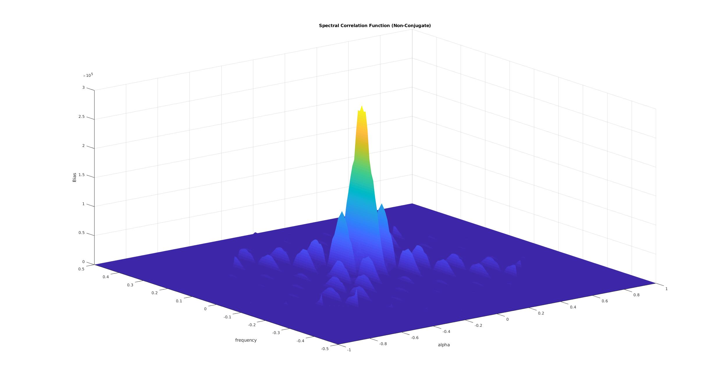
L = N’/16:

Reply
1. Chad Spooner says:
  
  September 24, 2021 at 12:36 pm
  
  I don’t think there is a lower bound on $L$ . I can’t see why there would be, from the equations or intuition. The matrices that I define above get bigger, however, as $L$ gets smaller, and that can be a computer-memory problem.
  
  As evidence that it is possible to use small $L$ , here are some results for various values of $L$ and $N^\prime = 128$ , $N = 16384$ , zero-padding factor of $2$ , and our usual rectangular-pulse BPSK signal as input ( $f_{bit} = 0.1$ ).
  
  First, the extracted bit-rate non-conjugate feature for each value of $L = 1, 2, 4, \ldots, 64$ :
  
  They are all pretty much the same. Now the CDPs for the same values of $L$ :
  
  L=1:
  
  L=2:
  
  L=4:
  
  L=32:
  
  L=64:
  
  That last CDP, for $L=64 = N^\prime/2$ shows the leakage problem.
  
  What were $N$ and $N^\prime$ for your plots above?
  
  Reply
Ruobin Sun says:

December 1, 2019 at 7:57 am

Hi Prof. Spooner

I followed your instruct to reproduce the FAM estimator. I found my result has magnitude difference of you plots. Am I right to use the fft.m function in Matlab to implement the two DFT procedure? Does it need to divided some scaler of signal length?
Besides, how to compensate the energy difference of hamming window? Should the result divided by its energy like the PSD estimation? I saw you said in the comment that it is a empirical method. I am a little bit confused about that.

Reply
1. Chad Spooner says:
  
  December 10, 2019 at 8:13 am
  
  Thanks for stopping by the CSP Blog Ruobin! And for your keen interest in the FAM.
  
  Am I right to use the fft.m function in Matlab to implement the two DFT procedure?
  
  Yes.
  
  Does it need to divided some scaler of signal length?
  
  Well, there are various scale factors involved in the computation, but you can apply them all at the same time toward the end of the computation. In my implementation, I don’t directly scale the output of either of the kinds of FFTs that are involved in the FAM.
  
  Besides, how to compensate the energy difference of hamming window? Should the result divided by its energy like the PSD estimation? I saw you said in the comment that it is a empirical method. I am a little bit confused about that.
  
  It is a good question. I don’t have a precise mathematical answer (oops!), but you can use an input with a known PSD (use the TSM or FSM to figure that out, they are much easier to deal with than the FAM or SSCA), and then find the PSD component of the FAM output. Figure out the appropriate scaling factor to make them match. If you apply all the scaling factors at the end, the combined factor depends on the window, any zero-padding you do, the length of the data N, the number of channels N’, and L.
  
  What have you tried?
  
  Reply
Hari prasad says:

December 30, 2019 at 5:02 am

Hi sir , Thanks for detailed information on FAM, I have gone through this whole post ,Just to confirm that my understanding is correct or not

After step 4 , I have a matrix P*N’^2 ,the elements in that matrix is nothing but scf correlation magnitudes. Now i need to find the corresponding elements in matrix belongs to what ( alpha and freq) ? All the elements in matrix is not required. We need to find only set of (alpha and freq) and corresponding correlation magnitudes which falls in principle region.
the principle region is nothing but -0.5 < f (+ or -) alpha/2 < 0.5

Is my understanding is correct ? Please clarify so that i can move further

Reply
1. Chad Spooner says:
  
  December 30, 2019 at 8:22 am
  
  Yes, that is correct. Have you tried to make the association? Don’t forget to use a simple, well-understood signal so you can know when the algorithm produces correct results for all $f$ and $\alpha$ in the principal domain.
  
  Reply
  1. Hari prasad says:
    
    January 2, 2020 at 12:15 am
    
    Hi sir , I have one more query regarding the complex demodulate
    If we analyse the complex demodulate equation , i felt it is convolution between hamming window a(r) and x(r)*exp(-j*2*pi*f*n*Ts). What is ur comment on that ?
    
    Reply
Hari prasad says:

January 2, 2020 at 3:58 am

Sir,
In the above comment section

Chen says:
August 28, 2019 at 5:29 pm

Chen has posted code for FAM , In that while calculating cyclic frequencies for associating scd estimates to (f,alpha) he used the equation
cyclefre=CF*fs/NN+dalpha*linspace(-N/NN,N/NN-1,2048);

as per definition (fk-fl) + q*del_alpha , where q ranges from (-P/2 to P/2 -1) or (0 to P-1) .
But i felt in that code he has not used as per definition . Is it correct of using that equation?
Please give ur suggestions on this

Reply
1. Chad Spooner says:
  
  January 5, 2020 at 4:57 pm
  
  I’m not sure; did you try it? What was the result?
  
  Reply
  1. Hari prasad says:
    
    January 5, 2020 at 10:50 pm
    
    May be he want to represent cyclic frequency range (-P/4 to P/4) ,that’s y he used linspace(-N/NN,N/NN-1,2048)
    where N = L*P , L = NN/4 , so N/NN = P/4 . Any way it is giving correct result.
    
    I have a question regarding this ,when i was doing this exercise , i found some of the cycle frequencies are overlapping if i am using (fk-fl) + q*del_alpha ,where q defines (-P/2 to P/2 -1) , but if used range of q from (-P/4 to P/4-1) , no overlapping of cyclic frequencies for set of freq(fk,fl).
    
    which is the correct method ,should we take q values in (-P/2 to P/2 -1) or (-P/4 to P/4-1)
    
    So please give ur comments on this
    
    Reply
Nick says:

July 21, 2020 at 3:00 pm

Hi Chad,

Many thanks and appreciation for all the knowledge you’ve shared on this blog. I am working on a project and I have implemented the FAM method that you’ve described above in MATLAB. Everything seems to be working fine, but there is an abnormality that I am curious if you have any insight about.

I am running the FAM method on a BPSK signal with fc = 0.05 and T_bits = 10. When I run the algorithm, I get SCF plots that look very similar in shape to the examples you have shown here. Based on your work, I expected the main peak of the SCF plot to occur at an alpha value of 0 for the non-conjugate SCF, and at an alpha value of 0.1 (2*fc) for the conjugate SCF. However, these peaks occur at alpha = 0.0625 and 0.1625, respectively. That is, both values are 0.0625 higher than expected.

Furthermore, I realized that tweaking the value of N’ in the MATLAB code affects this value. The first test case I ran had N’ = 32, just as in your example. This corresponds to a value of 2/N’ = 0.0625. When I increase the value of N’ to 64, the unexpected offset decreases to 0.03127, which is also roughly 2/N’. That is, the peaks for the conjugate and non-conjugate plots are 0.03127 and 0.13127, respectively.

I suspect that this is simply some sort of quantization error that occurs when the signal is split into subblocks? Do you have any further insight as to what could be causing this offset?

Cheers!
Nick

Reply
1. Chad Spooner says:
  
  July 21, 2020 at 3:28 pm
  
  Thanks for checking out the CSP Blog, Nick, and for the comment. It is likely this problem is, or will be, shared by other readers, so I appreciate you setting in down in writing here.
  
  Based on the sketch of the problem you provided, I think the most likely cause of your problem is an error in how the FAM outputs are associated with ordered pairs $(f, \alpha)$ (Step 5). When implemented correctly, the FAM will not shift the features in cycle frequency–you’ll see the conjugate peak at $\alpha = 2f_c$ for all values of $N$ and $N^\prime$ (except very small values of these parameters, which don’t permit decent estimation because insufficient “cycles” of the underlying periodic statistics are observed).
  
  My hint in the previous paragraph is strongly dependent on
  
  … I get SCF plots that look very similar in shape to the examples you have shown here.
  
  being accurate for each of the values of $N^\prime$ that you’ve tried. That is, it is really true that the shapes of your spectral correlation slices correspond to the shapes in the Blog.
  
  Reply
  1. Nick says:
    
    July 23, 2020 at 11:24 am
    
    Hi Chad,
    
    Thanks for your response. I’ve done some more digging, and I have determined that the offset is actually related to the value L, which you’ve defined as N’/4 in your example. I did some testing to confirm that the results are not related to the values of N, N’, or P, other parameters defined in the example.
    
    I also worked through all the places in my code where the value of L is used. I tried externally tweaking their usage in a variety of ways, but none of my changes affected the output. So I am unsure how I am misusing the property L to cause this error.
    
    Regarding Step 5 that you’ve specifically mentioned, I can correct the error by changing equation (6) to be alpha_i = f_k – f_l – 1/(2L). This -1/(2L) term corrects the plot. However, I am at a loss as to why this would correct the error. Do you have any insight into this occurrence?
    
    Thanks again!
    Nick
    
    Reply
    1. Chad Spooner says:
      
      July 23, 2020 at 3:54 pm
      
      Regarding Step 5 that you’ve specifically mentioned, I can correct the error by changing equation (6) to be $\alpha_i = f_k - f_l - 1/(2L).$ This $-1/(2L)$ term corrects the plot. However, I am at a loss as to why this would correct the error. Do you have any insight into this occurrence?
      
      Not yet. I can confirm that my FAM code doesn’t use $L$ much except that $P$ is a function of $L$ . When I do Step 5, I don’t explicitly use $L$ . I explicitly use $L$ when I create the hopped Fourier transforms (channelization) at the start of the algorithm, and it determines $P$ through $P = N/L$ .
      
      I revisited my FAM examples for this post, and did some further examples for variable $L$ with fixed $N$ and $N^\prime$ . Looking at the non-conjugate spectral correlation slice for $\alpha = 0.1$ (staying with our usual rectangular-pulse BPSK signal), I get this result for $N=16384$ and $N^\prime = 128$ :
      
      and the following sequence of cyclic-domain profiles:
      
      $L = 4$
      
      $L = 8$
      
      $L = 16$
      
      $L = 32$
      
      $L = 64$
      
      Reply
      1. Nick says:
        
        July 24, 2020 at 9:39 am
        
        For those who may be reading this having a similar issue, Chad was able to find the error in my code. It turns out that I was performing an fftshift as part of Step 4 of the process, but equation (8) produces an unshifted cycle frequency vector. This discrepancy was the cause of mismatch between the alpha values.
        
        To reiterate, Step 4 should perform an FFT, but not a shifted FFT. The instructions above do not call for a shifted FFT, but for some reason I used that in my code by mistake. This fixed my issue.
Nick says:

August 3, 2020 at 8:26 am

Hi Chad,

I am having another issue with my implementation of the FAM method. I am now working with real signal data from a capture, so in an attempt to generalize my algorithm, I have set `N = length(y_of_t)`. However, I then crash the algorithm when I try to index the final `output_scf`.

What happens is that `alpha_end-alpha_start+1` is greater than `P_blocks`, which is the length of a row of `SCF_estimate`.

Any insight you have would be appreciated. I will happily provide my code if it would be helpful to understand what I’m trying to do.

Thanks,
Nick

Reply
1. Chad Spooner says:
  
  August 3, 2020 at 9:01 am
  
  What happens is that `alpha_end-alpha_start+1` is greater than `P_blocks`, which is the length of a row of `SCF_estimate`.
  
  It sounds like there is an off-by-one type of error. I suggest truncating your captured data so that its length is dyadic and retry the FAM with this truncated data. If it works fine, then you are likely off by one somewhere due to the inconsistent use of things like floor.m and ceil.m. Let me know how that turns out.
  
  Reply
  1. Nick says:
    
    August 3, 2020 at 9:34 am
    
    Hi Chad,
    
    By dyadic, you mean of length 2^n, correct? You were right. Truncating my data in this way prevented my error.
    
    Does this mean there is an error somewhere in my code, or is it just a limitation of the algorithm that it works best with dyadic input?
    
    Thanks,
    Nick
    
    Reply
    1. Chad Spooner says:
      
      August 3, 2020 at 10:05 am
      
      Yes, I meant a power of two. So I think this means there is an error in the code involving division and rounding of some sort.
      
      You can try to make your code work for arbitrary N, or you can check the value of N at the top of the function and either zero pad to a dyadic number of samples or truncate to a dyadic number of samples.
      
      Reply
      1. Nick says:
        
        August 3, 2020 at 10:31 am
        
        It seems easier to zero pad/truncate. Are both methods equivalent?
        
        Thank you so much for your help.
      2. Chad Spooner says:
        
        August 3, 2020 at 10:56 am
        
        No, as you might imagine, truncating will reduce performance somewhat due to smaller block size in the resolution product. But it might be preferable in some situations, such as when the number of samples you have is just a bit larger than a dyadic number. Say you have 8200 samples. Then truncating to 8192 is a small data loss, whereas zero padding up to 16384 would incur an increase in computational cost without significant estimator-quality benefit.
Alex says:

June 27, 2022 at 9:54 pm

Dear Chad Spooner,
I came across your article when I was learning FAM, I had a problem trying to reproduce Figure 1, I know if my code is wrong or if it is different from your code theory.Looking forward to your reply.

Here is the source code.

%%%%%%%%%%%%%%%%%%%%%%%%%%%%%%%%%%%%%%
%%% Appendix B. function Auto-FAM %%%

%%%%%%%%%%%%%%%%%%%%%%%%%%%%%%%%%%%%%%
function [Sx,alphao,fo]=autofam(x,fs,df,dalpha)
%AUTOFAM(X,FS,DF,DALPHA) computes the spectral auto-correlation density function estimate of the signal X, by using the FFT Accumulation Method (FAM).
%Make sure that DF is much bigger than DALPHA in order to have a reliable estimate.
%AUTOFAM(X,FS,DF,DALPHA)

%INPUTS:
%x-input column vector;
%FS-sampling rate;
%DF- desired frequency resolution;
%DALPHA – desired cyclic frequency resolution.
%OUTPUTS:
%SX – spectral correlation density function estimate；
%ALPHAO – cyclic frequency;
%FO – spectrum frequency.
%
%Author: E.L.Da Costa,9/28/95.
if nargin~= 4
error(‘Wrong number of arguments.’);%Wrong number of arguments.
end
%%%%%%%%%%%%%%%%%%%%%%%%%%%
% Definition of Parameters

%%%%%%%%%%%%%%%%%%%%%%%%%%%
Np=pow2(nextpow2(fs/df)); % Number of input channels, defined by the desired frequency
% Np=fs/df, where fs is the original data sampling rate.
% It must be a power of 2 to avoid truncation or zero-padding in the FFT routines；
%
L=Np/4; % Offset between points in the same column at consecutive rows in the same channelization matrix.
% It should be chosen to be less than or equal to Np/4;
%
P=pow2(nextpow2(fs/dalpha/L)); %Number of rows formed in the channelization matrix, defined by the desired cyclic frequency resolution (dalpha) as follows:

%P=fs/dalpha/L.It must be a power of 2；
%
N=P*L; % Total number of points in the input data.
%
%%%%%%%%%%%%%%%%%%%%%%%%
% Input Channelization %
%%%%%%%%%%%%%%%%%%%%%%%%
if length(x)N
x=x(1:N);
end
NN=(P-1)*L+Np;
xx=x;
xx(NN)=0;
xx=xx(:);
X=zeros(Np,P);
for k=0:P-1
X(:,k+1)=xx(k*L+1:k*L+Np);
end
%%%%%%%%%%%%%
% Windowing %
%%%%%%%%%%%%%
a=hamming(Np);
XW=diag(a)*X;
XW=X;
%%%%%%%%%%%%%
% First FFT %
%%%%%%%%%%%%%
XF1=fft(XW);
XF1=fftshift(XF1);
XF1=[XF1(:,P/2+1:P) XF1(:,1:P/2)];
%%%%%%%%%%%%%%%%%%
% Downconversion %
%%%%%%%%%%%%%%%%%%
E=zeros(Np,P);
for k=-Np/2:Np/2-1
for m=0:P-1
E(k+Np/2+1,m+1)=exp(-i*2*pi*k*m*L/Np);
end
end
XD=XF1.*E;
XD=conj(XD’);
%%%%%%%%%%%%%%%%%%
% Multiplication %
%%%%%%%%%%%%%%%%%%
XM=zeros(P,Np^2);
for k=1:Np
for l=1:Np
XM(:,(k-1)*Np+1)=(XD(:,k).*conj(XD(:,1)));
end
end
%%%%%%%%%%%%%%
% Second FFT %
%%%%%%%%%%%%%%
XF2=fft(XM);
XF2=fftshift(XF2);
XF2=[XF2(:,Np^2/2+1:Np^2) XF2(:,1:Np^2/2)];
XF2=XF2(P/4:3*P/4,:);
M=abs(XF2);
alphao=-1:1/N:1;
fo=-.5:1/Np:.5;
Sx=zeros(Np+1,2*N+1);
for k1=1:P/2+1
for k2=1:Np^2
if rem(k2,Np)==0
l=Np/2-1;
else
l=rem(k2,Np)-Np/2-1;
end
k=ceil(k2/Np)-Np/2-1;
p=k1-P/4-1;
alpha=(k-1)/Np+(p-1)/L/P;
f=(k+1)/2/Np;
if alpha1
k2=k2+1;
elseif f.5
k2=k2+1;
else
kk=1+Np*(f+.5);
ll=1+N*(alpha+1);
Sx(kk,ll)=M(k1,k2);
end
end
end

%%%%%%%%%%%%%%%%%%%%%%%%%%%%%%%%%%%%%%
%%% APPENDIX F. Plotting routines %%%

%%%%%%%%%%%%%%%%%%%%%%%%%%%%%%%%%%%%%%
%%%%%%%%%%%%%%
%Surface Plot%
%%%%%%%%%%%%%%
figure(1)
surf1(alphao,fo,Sx);
view(-37.5,60);%
title( ‘SCD estimate using FAM’ );
xlabel( ‘alpha’ );
ylabel( ‘f’ );
zlabe1(‘Sx ‘);
%%%%%%%%%%%%%%
%Contour Plot%
%%%%%%%%%%%%%%
figure(2)
contour(alphao,fo,Sx);
xlabel(‘alpha(Hz)’);
ylabel(‘f(Hz)’);
%%%%%%%%%%%%%%%%%%%%%
%Cross-Section Plots%
%%%%%%%%%%%%%%%%%%%%%
figure(3)
plot(fo, Sx(:,1+N*(alpha/fs+1) ) ); % alpha is the desired cyclic
% frequency.
xlabel(‘f(Hz)’);
ylabel(‘Sx(alpha)’);

Reply
1. Chad Spooner says:
  
  June 28, 2022 at 11:17 am
  
  Thanks for the comment Alex!
  
  This doesn’t look like your code (different author). However, can you describe in some detail how your results are not matching mine? Some people here at the CSP Blog have used imgur to show me plots because WordPress won’t allow commenters to include images in comments.
  
  Reply
Mo says:

September 22, 2022 at 11:13 am

Dr. Spooner:

First off, thank you for the brilliant resource(s) you’ve put together in this blog. I’ve learned a ton, and look forward to learning more!

I’m attempting to use a pre-built FFT Accumulation Method method to detect cycle frequencies in a Python-based setting. The SCF estimations it produces match your provided rectangular BPSK signal reference. In attempting to compute the coherence for use in thresholding cycle frequencies, I’ve found that the peak coherence magnitudes can reach well over 100. Do you have any insight into where I might be going wrong? I’ve reproduced the coherence code below, and plots of the f=0 column of the FAM-estimated SCF and coherence matrix. In the examples below, I’ve chosen N’ (Np in the code below) = 32, P = 4096 and L=8.

Code:
def compute_coherence_matrix(self):
delta_f = 1.00 / (2*self.Np)
delta_a = 1.00 / (self.P*self.L)

# Interpolate the existing PSD row to get a closer estimate

# Spectral FFT bin 0 is -0.5 Hz, normalized
for scf_column in range(2*self.Np):

# Cyclic FFT bin 0 is -1.0 Hz, normalized
for scf_row in range(2*self.P*self.L):

f_spectral = (scf_column*delta_f – 0.5)
alpha = (scf_row*delta_a – 1.00)

# Step 1: compute interpolation for self.fam_scf[self.P*self.L, f – a*delta_a]
S_f_minus_a = np.interp(f_spectral – (alpha/2.00), self.spectral_freqs, self.fam_scf[self.P*self.L – 1 + self.cyclic_offset], left=np.inf, right=np.inf)

# Step 2: compute interpolation for self.fam_scf[self.P*self.L, f + a*delta_a]
S_f_plus_a = np.interp(f_spectral + (alpha/2.00), self.spectral_freqs, self.fam_scf[self.P*self.L – 1 + self.cyclic_offset], left=np.inf, right=np.inf)

# Step 3: compute coherence from interpolation points
self.fam_coherence[scf_row, scf_column] = self.fam_scf[scf_row, scf_column] / (math.sqrt(S_f_minus_a * S_f_plus_a))

Results:

FAM-estimated cycle frequencies (f=0 column of the SCF):
https://imgur.com/RPVTm56

Coherence estimation from the aforementioned FAM:
https://imgur.com/wpyln9S

Reply
1. Chad Spooner says:
  
  September 22, 2022 at 1:54 pm
  
  Welcome to the CSP Blog Mo! Thanks for the comment.
  
  Before we get to the coherence problem, let’s make sure the spectral correlation estimates are approximately correct.
  
  Here is the imgur image you posted for the FAM-produced spectral correlation:
  
  Now this isn’t exactly a cyclic-domain profile, which is not a slice across the cycle frequencies for a fixed spectral frequency, but is, apparently, the magnitudes of the spectral correlation for $f=0$ and all cycle frequencies produced by the FAM.
  
  But is it consistent with the expected values of the spectral correlation function for rectangular-pulse BPSK? First, I need to know if you processed the unchanged rectangular-pulse BPSK signal from the CSP Blog, which has bit rate of 0.1 and total power of 1.0 W (the noise power is 0.1, for a total power of 1.1). If so, the PSD has maximum of about 10 and the peak of the bit-rate non-conjugate spectral correlation function is about 3, as shown in the following two figures:
  
  Since the carrier frequency offset for the CSP Blog rectangular-pulse BPSK signal is 0.05, the $f=0$ slice of the SCF will not capture the maxima of the PSD and bit-rate SCF. Looking at the detailed spectral-correlation graphs for the CSP-Blog rectangular-pulse BPSK signal in the verification post, I find that the values of the PSD, 0.1, and 0.2 non-conjugate SCFs for $f=0$ should be about 3.2, 0, and 1.3, respectively. From your figure, I see about 1.2, 0.17, and 0.8, respectively.
  
  Are you using the unaltered (unit power for BPSK component) CSP Blog rectangular-pulse signal?
  
  It might be easier to compute and plot the CDP (find the maximum of the SCF and coherence magnitudes for each cycle frequency over all spectral frequencies) or plot the full magnitude surfaces.
  
  Reply
  1. Mo says:
    
    October 11, 2022 at 9:05 am
    
    After further experimentation, I think I have an SCF closer to your baseline results. My initial results used the wrong row of the resulting matrix for the PSD. In the code referenced above, steps 1) and 2) should index the FAM matrix row at self.P*self.L + self.cyclic_offset (I.E. the -1 should be omitted). After fixing the off-by-one error, my coherence results became MUCH more reasonable. To further refine my results, I increased the N’ and L parameters to 64 and 16 (respectively) takes my SCF and coherence results from this:
    
    SCF estimate: https://imgur.com/QJ4dVqp
    Coherence: https://imgur.com/L5PSURg
    
    To this:
    
    SCF estimate: https://imgur.com/zN57h1b
    Coherence: https://imgur.com/S4bd0a3
    
    Please note that these are the raw coherence and SCF results, without the filtering that removes the smaller-magnitude cycle frequencies. My results aren’t as smooth as the reference plots, but I believe you’ve addressed these artifacts elsewhere in this post. One final note: I used the following matplotlib example for this second set of plots: https://matplotlib.org/stable/gallery/mplot3d/polys3d.html. This represented a significant performance improvement over the other example I had used; hope this helps someone out!
    
    Reply
    1. Chad Spooner says:
      
      October 16, 2022 at 8:26 am
      
      Good progress!
      
      The imgur image of the new spectral correlation looks great.
      
      The image for the coherence looks wrong though:
      
      However, the plotting style makes it difficult to see the coherence functions for the key cycle frequencies of $0.1$ , $0.2$ , and $0.3$ . The strength and shapes of the functions for larger cycle frequencies ( $> 0.4$ ) do not appear to match those in the spectral coherence post. Can you plot the individual coherence slices for $0.1, 0.2, 0.3$ ? Do those match the corresponding plots in the verification post?
      
      Reply
Surya says:

October 31, 2022 at 10:51 pm

Hi Dr. Chad,
Thanks for great blog on Spectral Correlation Density.
I have a question regarding the Cycle Domain Plots. Of N_prime* N_prime*P SCF Estimates, do I simply pick all alpha points with corresponding spectral ferquency = 0 for cyclic Domain Plots?

Reply
1. Chad Spooner says:
  
  November 2, 2022 at 4:24 pm
  
  Hello Surya and welcome to the CSP Blog!
  
  The cyclic-domain profile (CDP) plots are formed by finding the maximum absolute value of the spectral correlation (or, alternatively, the spectral coherence) for each cycle frequency $\alpha$ over all spectral frequencies $f$ .
  
  So you have to search for the maximum over frequency for each unique cycle frequency in your estimator output.
  
  Does that help?
  
  Reply