Square-Root Raised-Cosine PSK/QAM

SRRC PSK and QAM signals form important components of more complicated real-world communication signals. Let’s look at their second-order cyclostationarity here.

Let’s look at a somewhat more realistic textbook signal: The PSK/QAM signal with independent and identically distributed symbols (IID) and a square-root raised-cosine (SRRC) pulse function. The SRRC pulse is used in many practical systems and in many theoretical and simulation studies. In this post, we’ll look at how the free parameter of the pulse function, called the roll-off parameter or excess bandwidth parameter, affects the power spectrum and the spectral correlation function.

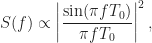
The problem with the rectangular pulse-shaping function in PSK and QAM signals is its low bandwidth efficiency. The PSD of the rectangular-pulse PSK signal has unlimited width because the PSD is proportional to the square of the pulse-function Fourier transform. That means the rectangular-pulse PSD is proportional to the square of the sinc() function

$\displaystyle S(f) \propto \left| \frac{\sin(\pi f T_0)}{\pi f T_0} \right|^2,$

where $1/T_0$ is the symbol rate. The sinc() function does not have bounded support. This simply means that there is no interval $[-F, F]$ , $F < \infty,$ such that $S(f)$ is zero outside the interval.

In practice, this means that the rectangular-pulse PSK/QAM signal possesses energy that interferes with signals in nearby (relative to the carrier frequency) frequency bands. Any duration-limited pulse function will possess this “infinite bandwidth” property, due to basic results in Fourier analysis: All duration-limited transformable functions have transforms with unbounded support.

So more sophisticated pulse functions must be sought. A popular one is the square-root raised-cosine (SRRC) pulse, which is related to the raised-cosine pulse. These pulse functions are parameterized by a number $R$ called the roll-off or excess-bandwidth parameter. It lies on the interval $[0, 1]$ and controls the bandwidth of the pulse transform, and therefore the bandwidth of the PSK/QAM signal as reflected by the width of the PSD.

If the symbol rate is 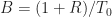$1/T_0$ , then the occupied bandwidth of a SRRC PSK/QAM signal is given by $\displaystyle B = (1 + R)/T_0$ . When $R=1$ , the occupied bandwidth is $2/T_0$ , or twice the symbol rate, and when $R=0,$ the occupied bandwidth is $1/T_0$ , or the symbol rate. All other valid values of $R$ produce occupied bandwidths between these two extremes.

Here at the CSP Blog we are interested in how the cyclic autocorrelation and spectral correlation function vary with $R$ . We will see that the non-conjugate functions vanish for $\alpha \neq 0$ when $R=0$ . That is, the non-conjugate symbol-rate-harmonic cycle frequencies are no longer cycle frequencies when $\latex R=0$. For BPSK, when $R=0$ only the doubled-carrier conjugate cycle frequency remains.

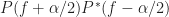
Mathematically, recall that the non-conjugate spectral correlation function for QAM/PSK is proportional to a shifted product of pulse transforms. In particular, suppose the pulse function is $p(t)$ . It has Fourier transform $P(f)$ . The non-conjugate spectral correlation function for digital PSK/QAM has the property

$\displaystyle S_s^\alpha (f) \propto P(f+\alpha/2)P^*(f-\alpha/2), \hfill (1)$

assuming that the signal is at complex baseband (the carrier frequency is zero). Now, the transform $P(f)$ has width $(1+R)/T_0$ and is restricted to the interval

$\displaystyle \left[\frac{-(1+R)}{2T_0}\ \ \frac{(1+R)}{2T_0}\right]$

(remember, the carrier is zero here).

First consider $\alpha = 0$ , the PSD. We have

$S_s^0(f) \propto | P(f) |^2, \hfill (2)$

and no matter how narrow $P(f)$ becomes, as long as it has some non-zero width, the PSD will not be zero for all frequencies. Next consider $\alpha = 1/T_0$ , the non-conjugate symbol-rate feature,

$S_s^{1/T_0} (f) \propto P(f+1/2T_0)P^*(f-1/2T_0). \hfill (3)$

Here the pulse transform $P(f)$ is shifted up by half the cycle frequency and down by half the cycle frequency and the two shifted transforms are multiplied together. If $R=0,$ then the two shifted pulse transforms do not overlap, and the spectral correlation function is zero for all frequencies $f$ for this cycle frequency. When $R > 0,$ there is some overlap, and the function is not zero everywhere. The situation for $R=0$ is illustrated here in Figure 1:

zero_ebw_pulse_overlap — Figure 1. Illustration of the effect of the SRRC roll-off factor on the non-conjugate spectral correlation function, which is proportional to $P(f+\alpha/2)P^*(f-\alpha/2)$ .

Figure 1. Illustration of the effect of the SRRC roll-off factor on the non-conjugate spectral correlation function, which is proportional to $P(f+\alpha/2)P^*(f-\alpha/2)$ .

Generating SRRC Signals

If we had a way to numerically evaluate the pulse function $p(t)$ , we could convolve it with an impulse train to obtain the modulated SRRC signal. The impulse train contains impulses spaced by $T_0$ samples, and each is multiplied by a complex symbol value drawn from the appropriate constellation (BPSK, 16QAM, etc.). I do this for a rectangular pulse $p(t)$ in this script.

The pulse function $p(t)$ and its transform $P(f)$ can be found on the web in various places. So one can program a function to create the pulse using C, MATLAB, etc. MATLAB also has a function to do this for us called rcosdesign.m. Here is a function that produces a SRRC BPSK signal by calling rcosdesign.m:

function [bpsk] = make_bpsk_srrc (num_syms, samples_per_sym, rolloff)
% function [bpsk] = make_bpsk_srrc (num_syms, samples_per_sym, rolloff)
%
% Create a BPSK signal with independent and identically distributed bits
% and a pulse function that is a square-root raised cosine pulse with
% roll-off parameter rolloff. The symbol (bit) rate is Rb =
% 1/samples_per_sym and the carrier frequency is zero. No noise is added.
% The calling program can frequency shift the returned signal to implement
% a carrier frequency and add noise as desired.
%
% The Nyquist bandwidth for a signal with rate Rb is Rb. The occupied
% bandwidth of the generated signal is (1 + rolloff)Rb, so that when
% rolloff is zero, the signal occupies its Nyquist bandwidth and when
% rolloff is one, the signal occupies twice its Nyquist bandwidth.
%
% num_syms and samples_per_sym must be positive integers.
%
% Chad M. Spooner
% May 2016

% Error checking.

if (nargin < 3)
   fprintf (‘make_bpsk_srrc: Insufficient arguments to function\n’);
   help make_bpsk_srrc;
   return;
end

if ( (rolloff < 0) || (rolloff > 1.0) )
   fprintf (‘make_bpsk_srrc: rolloff parameter must lie in [0.0, 1.0]\n’);
   help make_bpsk_srrc;
   return;
end

if (round(num_syms) ~= num_syms)
   fprintf (‘make_bpsk_srrc: num_syms must be a positive integer\n’);
   help make_bpsk_srrc;
   return;
end

if (round(samples_per_sym) ~= samples_per_sym)
   fprintf (‘make_bpsk_srrc: samples_per_sym must be a positive integer\n’);
   help make_bpsk_srrc;
   return;
end

% Create a random bit sequence.

bit_seq = randi([0 1], [1 num_syms]);

% Convert the {0, 1} bits into {-1, 1} symbols.

sym_seq = 2*bit_seq – 1;
zero_mat = zeros((samples_per_sym – 1), num_syms);
sym_seq = [sym_seq ; zero_mat];
sym_seq = reshape(sym_seq, 1, samples_per_sym*num_syms);

% Create the pulse function.

p_of_t = rcosdesign (rolloff, 30, samples_per_sym);

% Convolve bit sequence with pulse function.

s_of_t = filter(p_of_t, [1], sym_seq);

% Plot time-domain waveform.

figure(1);
hp = plot(real(s_of_t(1:400)));
hold on;
set(hp, ‘linewidth’, 2);
hp = plot(imag(s_of_t(1:400)), ‘-g’);
set(hp, ‘linewidth’, 2);
grid on;
hold off;
xlabel(‘Sample Index’);
ylabel(‘Signal Amplitude’);
title(‘Time-Domain Plot of SRRC-Pulse BPSK’);
set(gca, ‘ylim’, [-0.6 0.6]);
legend (‘Real Part’, ‘Imag Part’);
print -djpeg99 ‘srrc_bpsk_time_domain.jpg’

% Save the created signal.

% write_binary (‘srrc_bpsk_matlab.tim’, 2, s_of_t);

bpsk = s_of_t;

return

This script can be found (as a .doc file, just rename to an m-file locally) here. In the remainder of this post, I present some power spectra and spectral correlation functions for SRRC BPSK signals generated using the MATLAB and C methods, as well as some ideal functions from theory.

Power Spectra and Spectral Correlation Functions

The ideal spectral correlation function can be computed for SRRC PSK/QAM, and is readily numerically evaluated. In the six graphs that follow, the symbol rate for the SRRC BPSK signal is $1/T_0 = 1/5$ and the carrier offset is zero. The ideal power spectra as a function of roll-off $R$ and frequency $f$ are shown here:

theory_srrc_bpsk_psds — Figure 2. Ideal SRRC BPSK power spectra as a function of the SRRC roll-off factor $R$ . These are obtained from numerical evaluation of theoretical formulas.

Figure 2. Ideal SRRC BPSK power spectra as a function of the SRRC roll-off factor $R$ . These are obtained from numerical evaluation of theoretical formulas.

The corresponding estimated PSDs from the CSP Blog’s C-language communication-signal simulator are shown next:

srrc_bpsk_psds_scene — Figure 3. Estimated power spectra for SRRC BPSK corresponding to the theoretical power spectra in Figure 2. The signals are generated using a custom CSP-Blog C program for general communication-signal simulation.

and the estimated PSDs for the MATLAB generator are:

srrc_bpsk_psds_matlab — Figure 4. Estimated power spectra for SRRC BPSK corresponding to the theoretical power spectra in Figure 2. The signals are generated using MATLAB functions.

The sequence of plots for the non-conjugate SCF for $\alpha = 1/T_0$ are shown next:

theory_srrc_bpsk_scfs — Figure 5. Ideal SRRC BPSK non-conjugate spectral correlation function magnitudes a function of the SRRC roll-off factor $R$ . These are obtained from numerical evaluation of theoretical formulas.

Figure 5. Ideal SRRC BPSK non-conjugate spectral correlation function magnitudes a function of the SRRC roll-off factor $R$ . These are obtained from numerical evaluation of theoretical formulas.

srrc_bpsk_nc_scfs_scene — Figure 6. Estimated non-conjugate spectral correlation function magnitudes for SRRC BPSK corresponding to the theoretical power spectra in Figure 2. The signals are generated using a custom CSP-Blog C program for general communication-signal simulation.

srrc_bpsk_nc_scfs_matlab — Figure 7. Estimated non-conjugate spectral correlation function magnitudes for SRRC BPSK corresponding to the theoretical power spectra in Figure 2. The signals are generated using MATLAB functions.

The measured functions differ somewhat from the ideal, but they generally agree. The difference of most concern is for the MATLAB-based case of $R=0$ . But perhaps the Mathworks did not sufficiently test the rather degenerate case of $R=0$ , or I’m somehow using it incorrectly.

There are practical signals, by the way, that correspond to $R=0$ , such as the duobinary signals (The Literature [R44]). However, the transmitted symbols are no longer IID. Also, as mentioned in my introductory post on higher-order cyclostationarity, such duobinary signals do possess exploitable higher-order features.

Finally, let’s look at a sequence of complete estimated spectral correlation functions as a function of the roll-off $R$ . Here the symbol rate is $1/T_0 = 1/5$ , the carrier frequency is $0.05$ , and the signals are generated using the CSP-Blog C program.

ww_scf_bpsk_1.0 — Figure 8. Estimated spectral correlation functions for cycle frequencies exhibited by square-root raised-cosine BPSK. Here the SRRC roll-off factor is 1.0. The bit rate is 0.2 and the carrier offset is 0.05.

ww_scf_bpsk_0.5 — Figure 9. Estimated spectral correlation functions for cycle frequencies exhibited by square-root raised-cosine BPSK. Here the SRRC roll-off factor is 0.5. The bit rate is 0.2 and the carrier offset is 0.05.

ww_scf_bpsk_0.35 — Figure 10. Estimated spectral correlation functions for cycle frequencies exhibited by square-root raised-cosine BPSK. Here the SRRC roll-off factor is 0.35. The bit rate is 0.2 and the carrier offset is 0.05.

ww_scf_bpsk_0.20 — Figure 11. Estimated spectral correlation functions for cycle frequencies exhibited by square-root raised-cosine BPSK. Here the SRRC roll-off factor is 0.20. The bit rate is 0.2 and the carrier offset is 0.05.

ww_scf_bpsk_0.10 — Figure 12. Estimated spectral correlation functions for cycle frequencies exhibited by square-root raised-cosine BPSK. Here the SRRC roll-off factor is 0.1. The bit rate is 0.2 and the carrier offset is 0.05.

ww_scf_bpsk_0.0 — Figure 13. Estimated spectral correlation functions for cycle frequencies exhibited by square-root raised-cosine BPSK. Here the SRRC roll-off factor is 0.0. The bit rate is 0.2 and the carrier offset is 0.05. This choice of roll-off results in a single non-conjugate cycle frequency (zero, corresponding to the PSD) and a single conjugate cycle frequency (0.1, the doubled carrier). All other features, seen for $R > 0$ , vanish.

Figure 13. Estimated spectral correlation functions for cycle frequencies exhibited by square-root raised-cosine BPSK. Here the SRRC roll-off factor is 0.0. The bit rate is 0.2 and the carrier offset is 0.05. This choice of roll-off results in a single non-conjugate cycle frequency (zero, corresponding to the PSD) and a single conjugate cycle frequency (0.1, the doubled carrier). All other features, seen for $R > 0$ , vanish.

The bottom line for CSP is that as the excess bandwidth (SRRC roll-off parameter) becomes smaller and smaller in order to force the transmitted signal into an ever-more-narrow frequency slot, the ability of CSP detectors to reliably detect the non-conjugate symbol-rate feature steadily decreases. Eventually, when the excess bandwidth is zero (SRRC roll-off parameter is zero), the BPSK signal looks like conventional AM, and the non-BPSK SRRC QAM/PSK signals are stationary of order two. They all still have higher-order cyclostationarity, though!

Author: Chad Spooner

I'm a signal processing researcher specializing in cyclostationary signal processing (CSP) for communication signals. I hope to use this blog to help others with their cyclo-projects and to learn more about how CSP is being used and extended worldwide. View all posts by Chad Spooner

9 thoughts on “Square-Root Raised-Cosine PSK/QAM”

Chen says:

September 22, 2019 at 1:43 am

Hi Chad
The paper “Cyclic Wiener Filtering: Theory and Method”, by Gardner, mentions an example of 200% excess bandwidth in part V, which means that the roll-off factor equals to 2. The example is conflict with your opinion that roll-off factor must be smaller than 1. Why?

Reply
1. Chad Spooner says:
  
  September 23, 2019 at 7:00 am
  
  I think Gardner’s large excess bandwidths in that paper are in conflict with a maximum square-root raised-cosine roll-off of 1.0 only if he is explicitly saying he is using square-root raised-cosine pulses. I don’t think he says that. So you can’t infer that the roll-off factor is 2 from his statement that the excess bandwidth is 200%. You could only do that in the context of square-root raised-cosine pulses.
  
  The excess bandwidth of a rectangular-pulse PSK/QAM signal is infinite, since the signal bandwidth is itself infinite. In fact, any time-limited pulse will result in an infinite bandwidth signal. You can also imagine just creating whatever pulse function you want in the frequency domain. Note that such pulses will unlikely meet the Nyquist intersymbol-interference-free criterion.
  
  It isn’t my opinion that the roll-off be less than or equal to 1.0, and greater than or equal to 0.0, it is in the definition of the pulse.
  
  Gardner is using signals with large excess bandwidth because they are favorable to the FREquency-SHift (FRESH) filtering technique he is advancing in the paper. The larger the excess bandwidth, the more cycle frequencies there are, and the wider each feature is in frequency, so the filter has more pairs of correlated spectral components to work with.
  
  Reply
2. Chen says:
  
  September 23, 2019 at 7:38 am
  
  If another pulse function is used, such as triangular function, the excess bandwidth will be larger than 100%, right?
  
  Reply
  1. Chen says:
    
    September 23, 2019 at 7:54 am
    
    Thanks for your reply, I understand what you said!
    
    Reply
  2. Chad Spooner says:
    
    September 23, 2019 at 8:14 am
    
    Yes, if the triangle is in the time-domain. Sometimes people talk about a triangular spectrum.
    
    Reply
John Snoap says:

March 9, 2021 at 4:54 pm

Hi Chad,

To avoid using MATLAB’s rcosdesign function for SRRC pulse shaping, I created my own function in MATLAB. After several different approaches, the one that seemed to work best was implementing the SRRC pulse shape in the time-domain using the formula found here https://en.wikipedia.org/wiki/Root-raised-cosine_filter. However, when I did this and estimated the PSD and SCF plots of the created SRRC BPSK signal, the plots were the same as MATLAB’s rcosdesign function produced! The pulse shapes they create are also quite similar, although not 100% identical.

Do you have any tips on how to better go about implementing the SRRC pulse shaping function? Should I try a frequency domain approach instead? My function currently has as inputs the roll-off factor (rolloff), the number of symbols (num_syms), and the number of samples per symbol (samples_per_sym); from which I create a “time” vector t = (-num_syms/2*samples_per_sym):1:((num_syms/2*samples_per_sym)-1);

From there I’m able to easily implement the pulse shaping function in the time-domain, but I’m not sure how to go about improving it so the PSD and SCF plots of an SRRC BPSK signal are more accurate.

Whenever you can get to this is fine, as this isn’t my main focus right now.

Thanks,
John

Reply
1. Chad Spooner says:
  
  March 10, 2021 at 10:47 am
  
  Hey John. Thanks for the thoughtful comment.
  
  Well, the first thing that comes to mind is that I am the one in the wrong, not MATLAB. So let’s not rule that out.
  
  What bothers me about the MATLAB results in the post is (1) the R=0 PSD has peaks on its two edges, and (2) the width of the measured SCF for R=1 and $\alpha=0.1$ exceeds its theoretical value of the BPSK bit rate. I think the extra energy near the PSD edges for R=0 helps explain the non-zero (and significant) feature for R=0 and $\alpha=0.1$ for MATLAB.
  
  The knob we can turn to try to force more accuracy is the number of symbols that the generated pulse spans. In the MATLAB function for SRRC signals that I posted here, I fixed the number of symbols that the pulse spans to 30. In my C code, I don’t take that approach–I generate a time-domain pulse that is long enough to satisfy a user-specifiable constraint on the ratio of the pulse at the edge to the maximum value of the pulse. In other words, I span sufficient symbols with the pulse so that it has decayed by at least an amount input by the user (say, 0.001).
  
  Reply
  1. John Snoap says:
    
    March 13, 2021 at 1:56 pm
    
    To try and improve MATLAB’s (and my) pulse shaping function, I went ahead and increased the number of symbols the generated pulse spans, before it had been 30, as you said, so let’s call it span = 30. When I increased the span, after filtering (or convolution) there was an issue that became more apparent at the beginning of the generated signal where the amplitude was essentially zero.
    
    There were a couple ways I got around this. One option was to initially generate more symbols by using
    
    num_syms = num_syms + span;
    
    and then after filtering, use:
    
    s_of_t = s_of_t(ceil(length(p_of_t)/2):end-floor(length(p_of_t)/2));
    
    As that would make the generated signal the correct size and remove the issue at the start of the generated signal.
    
    An easier way to handle this (instead of generating more symbols and then chopping off the ends) was to simply replace the filter command with:
    
    s_of_t = conv(sym_seq, p_of_t, ‘same’);
    
    As that will effectively generate a longer signal but then chop off the ends for you.
    
    Also, if you take the pulse shaping function generated by MATLAB and multiply it by sqrt(samples_per_sym), that will force your s_of_t to have unit power, and it causes MATLAB’s pulse to equal mine.
    
    However, after doing all this and trying span = 30, 300, 3000, and even 30000; the final generated signal remains (almost exactly) the same, as do its SCF plots. If I generate both a rectangular pulse shaped and SRRC pulse shaped BPSK signal and show them scaled to equal heights on the same plot, we can see the SRRC pulse shaped BPSK signal has rather jagged edges, although this seems to correspond to the samples_per_sym.
    
    Not sure if that provides any insight on the quality of the signal or not, but if I attempt to improve the smoothness of the pulse shaping function, the generated signal will no longer have a symbol rate of samples_per_sym. At the moment, I’m not sure what else to inspect/try. I’ll email the plots of the SRRC and Rect pulse signals to you, Chad, so you can post them if you think it helps.
    
    Reply
    1. Chad Spooner says:
      
      March 20, 2021 at 3:30 pm
      
      I’m not sure what is going on with MATLAB’s square-root raised-cosine generator, but I’m suspicious of it because as the roll-off goes to zero, the non-conjugate symbol-rate spectral correlation function does not vanish. But it should. When the pulse is such that it has an occupied bandwidth of less than or equal to the symbol rate, then there cannot be two distinct non-zero spectral components of the signal that are separated by the symbol rate! And that is what spectral correlation requires here. I also cannot force better behavior by varying the span in rcosdesign.m.
      
      Here is why I’m suspicious, in a nutshell. First, here are some more PSDs for the MATLAB-generated SRRC BPSK signal:
      
      and here are the corresponding PSDs for C-generated SRRC BPSK:
      
      Next, for these signals, I measured the peak spectral correlation and coherence magnitudes for the symbol-rate cycle frequency of 0.2:
      
      So the coherence and spectral-correlation peaks don’t go to zero as the bandwidth shrinks to 0.2. This makes me suspicious of the rcosdesign.m function in general, although it may be fine for larger roll-offs, and just suffers a problem for small roll-offs (and those near 1.0 as we saw in the post itself).
      
      Reply