Cyclostationarity of Frequency-Shift-Keyed Signals – Cyclostationary Signal Processing

Let’s get back to basics by looking at a large class of signals known as frequency-shift-keyed (FSK) signals. We will leave to the side, for the most part, the very large class of signals that goes by the name of continuous-phase modulation (CPM), which includes continuous-phase FSK (CPFSK), MSK, GMSK, and many more (The Literature [R188]-[R190]). Those are treated in My Papers [8], and in a future CSP Blog post.

Here we want to look at more conventional forms of FSK. These signal types don’t necessarily have a continuous phase function. They are generally easier to demodulate and are more robust to noise and interference than the more complicated CPM signal types, but generally have much lower spectral efficiency. They are like the rectangular-pulse PSK of the FSK/CPM world. But they are still used.

FSK Cycle Frequencies: Mathematical Approach

Three distinct types of frequency-shift-keyed (FSK) signals are
analyzed in this post. The analysis is directed at finding the set of potential cycle frequencies for each type of FSK signal for all orders and conjugation patterns by examining the cyclic temporal moment functions.

The FSK signals analyzed here are not constrained to exhibit a continuous phase function. The three types of signals arise from distinct models for the sequence of phase variables $\theta_k (f_k)$ in the generic complex-envelope FSK signal model given by The Literature [R1]

$\displaystyle s_c (t) = \sum_{k=-\infty}^\infty \exp \left( i2\pi f_k t +i\theta_k (f_k) \right) p(t - kT_0 - t_0), \hfill (1)$

where $f_k$ is a sequence of IID random variables drawn from the $M$ ary set $\{\omega_d \}_{d = 1}^M$ .

The first type of FSK signal corresponds to an independent and identically distributed (IID) phase-variable sequence ${\theta_k (f_k) = \theta_k}$ ,
where the distribution is uniform on the interval $[0, 2\pi)$ . Such an FSK signal is known as incoherent FSK (IFSK). The second type of FSK signal is known as carrier-phase-coherent FSK (CaPC FSK). For CaPC FSK, the phase sequence is dependent on $k$ only through the value of the frequency $f_k$ ,

$\displaystyle \theta_k (f_k) = \theta(f_k). \hfill (2)$

Thus, for CaPC FSK, the signal consists of bursts of randomly selected fixed-phase oscillator outputs. The third type of FSK signal is called clock-phase coherent FSK (ClPC FSK), and it is formed by setting the phase of the oscillator to a constant that depends on the transmitted frequency each time that frequency is selected for transmission. Thus, the phase variables are given by

$\displaystyle \theta_k (f_k) = -2\pi f_k (t_0 + kT_0) + \theta(f_k). \hfill (3)$

We analyze the three types of FSK separately next.

Incoherent FSK

The complex-envelope of the IFSK signal is given by

$\displaystyle s_c(t) = \sum_{-\infty}^\infty \exp \left( i2\pi f_k t + i \theta_k \right) p(t - kT_0 - t_0), \hfill (4)$

where ${\theta_k}$ is an IID sequence of continuous random phase-variables with uniform distribution on $[0, 2\pi)$ , and ${f_k}$ is an IID sequence of equiprobable frequencies drawn from the set of $M$ frequencies $\{\omega_d\}_{d=1}^M$ .

The IFSK signal can be represented as a random-pulse complex-valued PAM signal by simple manipulation,

$\displaystyle \begin{array}{lll} s_c(t) &=& \displaystyle \sum_{k=-\infty}^\infty e^{i\theta_k} e^{i2\pi f_k t} p(t -kT_0 - t_0) \hfill (5) \\ & = & \displaystyle \sum_{k=-\infty}^\infty e^{i\theta_k} e^{i2\pi f_k(t - kT_0 - t_0)} e^{i2\pi f_k (kT_0 + t_0)} p(t - kT_0 - t_0) \hfill (6)\\ &=& \displaystyle \sum_{k=-\infty}^\infty \left[ e^{i\theta_k} e^{i2\pi f_k (kT_0 + t_0)} \right] q_k (t - kT_0 - t_0) \hfill (7)\\&=& \displaystyle \sum_{k=-\infty}^\infty \left[ a_k e^{i2\pi f_k (kT_0 + t_0)} \right] q_k (t - kT_0 - t_0) \hfill (8) \\ &=& \displaystyle \sum_{k=-\infty}^\infty c_k q_k (t- kT_0 - t_0), \hfill (9) \end{array}$

where

$\displaystyle \begin{array}{lll} q(t) & \stackrel{\scriptscriptstyle \bigtriangleup}{=}\ & p(t) e^{i2\pi f_k t} \hfill (10) \\ a_k & \stackrel{\scriptscriptstyle \bigtriangleup}{=}\ & e^{i\theta_k} \hfill (11) \\ c_k & \stackrel{\scriptscriptstyle \bigtriangleup}{=}\ & a_k e^{i2\pi f_k (k T_0 + t_0)}. \hfill (12) \end{array}$

The moments $R_a (n,m)$ of the symbol sequence ${a_k}$ are nonzero only for $n = 2m$ , a result that follows easily from the properties of the phase sequence ${\theta_k}$ . It is also relatively easy to show that the moments $R_c (n,m)$ of the symbol sequence $c_k$ are identical to those for ${a_k}$ .

Because the pulse function and the symbols are both random, the formulas for digital QAM cumulants presented in the DQAM post do not apply. Let’s try to find the moment functions for the signal. The $n$ th-order temporal moment function is given by

$\displaystyle \begin{array}{lll} R_{s_c} (t, \boldsymbol{\tau}; n,m) & \stackrel{\scriptscriptstyle \bigtriangleup}{=}\ & \displaystyle E \left[ \prod_{j=1}^n s_c^{(*)_j} (t + \tau_j) \right] \hfill (13) \\ & = & \displaystyle E\left[ \prod_{j=1}^n \left( \sum_{k_j = -\infty}^\infty c_{k_j}^{(*)_j} q_{k_j}^{(*)_j} (t - k_j T_0 + \tau_j - t_0) \right) \right] \hfill (14) \\ & = & \displaystyle \sum_{k_1=-\infty}^\infty \cdots \sum_{k_n=-\infty}^\infty E\left[ \prod_{j=1}^n c_{k_j}^{(*)_j} \right] E\left[\prod_{j=1}^n q_{k_j}^{(*)_j} (t - k_j T_0 + \tau_j - t_0)\right]. \hfill (15) \end{array}$

The $n$ th-order moment of the symbols

$\displaystyle R_{\boldsymbol{c}} (n,m) \stackrel{\scriptscriptstyle \bigtriangleup}{=}\ E\left[ \prod_{j=1}^n c_{k_j}^{(*)_j} \right], \hfill (16)$

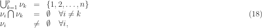
is a little tricky to evaluate. Let’s express the product as a product of products, each term of which involves one value of $k_j$ . To do this, we employ the notion of partitions once again,

$\displaystyle \prod_{j=1}^n c_{k_j}^{(*)_j} = \prod_{k=1}^p \left[ \prod_{j\in \nu_k} c_{k_{\nu_k}}^{(*)_j} \right], \hfill (17)$

where

$\displaystyle \begin{array}{lll} \bigcup_{k=1}^p \nu_k & = & \displaystyle \{1,2, \ldots, n\} \\ \nu_i \bigcap \nu_k & = & \displaystyle \emptyset \ \ \ \forall i \neq k \\ \nu_i & \neq & \emptyset \ \ \ \forall i, \end{array} \hfill (18)$

$k_{\nu_k}$ is the common value of $k_j$ for each $j \in \nu_k$ , and no two values of $k_{\nu_k}$ are equal. This notation includes all possible selections of indices for the symbols, from all equal to some index $k_0$ ( $p = 1$ ) to all distinct ( $p = n$ , $|\nu_k| = n_k = 1 \ \forall k$ ).

Because the symbols are independent, the moment is given by

$\displaystyle \begin{array}{lll} R_{\boldsymbol{c}} (n, m) & = & \displaystyle E \left[ \prod_{j=1}^n c_{k_j}^{(*)_j} \right] \\ & = & \displaystyle \prod_{k=1}^p E \left[ \prod_{j\in \nu_k} c_{k_{\nu_k}}^{(*)_j} \right]. \end{array} \hfill (19)$

For each expectation to be nonzero, we require that the order $n_k$ be even and be equal to $2m_k$ , where $m_k$ is equal to the number of conjugated factors in the $k$ th moment. Thus, we require that $n = 2m$ . The moment is given, therefore, by the following expression

$\displaystyle R_{\boldsymbol{c}} (n,m) = E \left[ \prod_{j=1}^n c_{k_j}^{(*)_j} \right] = \left\{ \begin{array}{ll} 1^p = 1, & n_k = 2m_k \ \ \forall k, \ \ n {\rm \ even}, \\ 0, & {\rm otherwise}. \end{array} \right. \hfill (20)$

The remaining analysis does not depend heavily on the particular set of indices that are chosen; a reasonable choice to focus on is the set in which all indices are equal: $k_1 = k_2 = \cdots = k_n = k$ . If there are $Z$ ways to partition the indices so that the resulting moment component is nonzero, then the moment function can be represented by the sum over these $Z$ components,

$\displaystyle R_{s_c} (t, \boldsymbol{\tau}; n,m) = \sum_{z = 1}^Z R_{s_z} (t, \boldsymbol{\tau}; n,m). \hfill(21)$

Let’s assume that $z=1$ corresponds to the case in which all indices are equal and find the corresponding moment component $R_{s_1} (t, \boldsymbol{\tau}; n,m)$ .

$\displaystyle \begin{array}{lll} R_{s_1} (t, \boldsymbol{\tau}; n,m) & = & \displaystyle \sum_{k=-\infty}^\infty E \left[ \prod_{j=1}^n c_k^{(*)_j} \right] E \left[ \prod_{j=1}^n q_k^{(*)_j} (t - kT_0 + \tau_j - t_0) \right] \\ & = & \displaystyle \left\{ \begin{array}{ll} \displaystyle{\sum_{k=-\infty}^\infty} E \left[ \displaystyle{\prod_{j=1}^n} q_k^{(*)_j} (t - kT_0 + \tau_j - t_0) \right], & n = 2m, \\ 0, & n \neq 2m. \end{array} \right. \end{array} \hfill (22)$

So, we are left with evaluating the moment function for the random pulse,

$\displaystyle R_q (t, \boldsymbol{\tau}; n, n/2) \stackrel{\scriptscriptstyle \bigtriangleup}{=}\ E \left[ q_k^{(*)_j} (t - kT_0 - t_0 + \tau_j) \right]. \hfill (23)$

This moment function is relatively easy to evaluate since the number of conjugations is equal to $n/2$ . The result is given by

$\displaystyle \begin{array}{lll} R_q (t, \boldsymbol{\tau}; n, n/2) & = & \displaystyle g(\boldsymbol{\tau};n) \prod_{j=1}^n p^{(*)_j} (t - kT_0 - t_0 + \tau_j), \end{array} \hfill (24)$

where

$\displaystyle \begin{array}{lll} g(\boldsymbol{\tau}; n) & \stackrel{\scriptscriptstyle \bigtriangleup}{=}\ & \displaystyle \frac{1}{M} \sum_{r=1}^M \exp(i2\pi \omega_r \tau_0), \\ \tau_0 & \stackrel{\scriptscriptstyle \bigtriangleup}{=}\ & \displaystyle \sum_{j=1}^n (-)_j \tau_j. \end{array} \hfill (25)$

Thus, the component of the moment function corresponding to identical indices is given by

$\displaystyle \begin{array}{lll} R_{s_1} (t, \boldsymbol{\tau}; n, n/2) & = & \displaystyle g(\boldsymbol{\tau};n) \sum_{k=-\infty}^\infty \left[ \prod_{j=1}^n p^{(*)_j} (t - kT_0 - t_0 + \tau_j) \right]. \end{array} \hfill (26)$

Note that this component is periodic in $t$ with period $T_0$ ; all other components possess this property as well. Therefore, the moment function for IFSK is periodic with period $T_0$ and is nonzero only for $n=2m$ . It follows that the cumulant function is also periodic with period $T_0$ and is nonzero only for $n=2m$ . In conclusion, the cycle frequencies for IFSK are limited to harmonics of the symbol rate for $n=2m$ for all even orders $n$ , which is the desired result of the analysis.

Carrier-Phase-Coherent FSK

For carrier-phase coherent FSK (CaPC FSK), the carrier phase variable $\theta_k (f_k)$ depends only on the value of $f_k$ and not explicitly on $k$ ,

$\displaystyle s_c (t) = \sum_{k=-\infty}^\infty \exp \left( i2\pi f_k t + i\theta (f_k) \right) p(t - kT_0 - t_0), \hfill (27)$

where $\theta (f_k)$ is equal to the constant $\theta (\omega_d)$ whenever $f_k = \omega_d$ , $d = 1, \ldots, M$ . Thus, this kind of FSK modulator transmits a burst of the output of one of $M$ continuously running oscillators with frequencies $\omega_d$ , $d=1, \ldots, M$ during each signaling interval.

We use straightforward analysis to find the temporal moment function for the CaPC FSK signal, which will allow us to determine the largest possible set of moment and cumulant cycle frequencies for the signal. The $n$ th-order temporal moment function is given by

$\displaystyle R_{s_c} (t, \boldsymbol{\tau}; n,m) = E\left[ \prod_{j=1}^n s_c^{(*)_j} (t + \tau_j) \right], \hfill (28)$

which, after some algebraic manipulation, can be expressed as

$\displaystyle \begin{array}{lll} R_s (t, \boldsymbol{\tau}; n,m) & = & \displaystyle E\left[ \sum_{k_1=-\infty}^\infty \cdots \sum_{k_n=-\infty}^\infty \Phi(t, p(t), \boldsymbol{\tau}; n,m) h(\boldsymbol{\theta};n,m) \left( \prod_{j=1}^n e^{(-)_j i2\pi f_{k_j} (t + \tau_j)}\right) \right], \end{array} \hfill (29)$

where

$\displaystyle \begin{array}{lll} h(\boldsymbol{\theta}; n,m) & \stackrel{\scriptscriptstyle \bigtriangleup}{=}\ & \displaystyle \prod_{j=1}^n e^{(-)_j i \theta(f_{k_j})} \\ \Phi (t, p(t), \boldsymbol{\tau}; n,m) & \stackrel{\scriptscriptstyle \bigtriangleup}{=}\ & \displaystyle \prod_{j=1}^n p^{(*)_j} (t - k_j T_0 - t_0 + \tau_j). \end{array} \hfill (30)$

The random quantities are those that involve the random symbols $f_k$ , so that the expectation can be moved inside the sums. However, as we saw in the case of IFSK, the value of the expectation depends on the nature of the indices $k_j$ . For $\{k_j\}_{j=1}^n$ distinct, the expectation simplifies to

$\displaystyle \begin{array}{lll} E\left[ h(\boldsymbol{\theta};n,m) \left( \prod_{j=1}^n e^{(-)_j i2\pi f_{k_j} (t + \tau_j)}\right) \right] & = & \displaystyle \prod_{j=1}^n \left[ \frac{1}{M} \sum_{r_j = 1}^M e^{(-)_j i \theta(\omega_{r_j})} e^{(-)_j i2\pi \omega_{r_j} (t + \tau_j)} \right]. \end{array} \hfill (31)$

Notice that the expectation results in the n-fold product of the sum of $M$ sine waves. At the other extreme, the values of the indices are equal, $k_j = k$ $\forall j$ , and the expectation simplifies to

$\displaystyle \begin{array}{lll} E\left[ h(\boldsymbol{\theta};n,m) \left( \prod_{j=1}^n e^{(-)_j i2\pi f_{k} (t + \tau_j)}\right) \right] & = & \displaystyle E\left[ \exp \left( i2\pi f_k \displaystyle{\sum_{j=1}^n} (-)_j (t + \tau_j) + i\displaystyle{\sum_{j=1}^n} (-)_j \theta(f_k) \right) \right] \\ & = & \displaystyle E\left[ \exp \left(i2\pi f_k \left([n-2m]t + \tau_0 \right) + i\displaystyle{\sum_{j=1}^n}(-)_j \theta(f_k) \right) \right] \\ & = & \displaystyle \frac{1}{M} \sum_{r=1}^M \exp \left( i2\pi \omega_r ([n-2m]t + \tau_0) + i(n-2m)\theta(\omega_r) \right), \end{array} \hfill (32)$

which is the sum of $M$ sine waves with frequencies given by $(n -2m)\omega_r$ . The other possibilities for the indices also result in the presence of additive sine-wave components. In fact, the notion of partitions is again of use here. The expectation yields sine-wave components with frequencies given by

$\displaystyle \beta_\rho = \sum_{j=1}^p (n_j - 2m_j)F_j, \hfill (33)$

where $F_j$ can be any of the $M$ frequencies $\{\omega_d\}_{d=1}^M$ , and $\rho$ denotes a partition of the index set ${1, 2, \ldots, n}$ with $p$ elements.

Since the function $\Phi()$ is periodic in $t$ with period $T_0$ for any choice of the indices $k_j$ , the actual set of moment cycle frequencies is given by

$\displaystyle \beta_\rho + k/T_0. \hfill (34)$

This is a large set of cycle frequencies. To demonstrate this, and to corroborate the cycle frequencies with those in The Literature [R1], let us compute the cycle frequencies for order $n=2$ for $M$ ary CaPC FSK.

For $n=2$ and $m=0$ , $m_j = 0$ for all partitions, and the cycle frequencies are given by

$\displaystyle \beta = \sum_{j=1}^p n_j F_j \pm k/T_0. \hfill (35)$

For $m = 1$ , the general formula applies,

$\displaystyle \beta = \sum_{j=1}^p (n_j - 2m_j)F_j \pm k/T_0. \hfill (36)$

Table 1 provides the cycle frequencies as a function of the partitions for the two values of $m$ . The derived cycle frequencies herein match those in The Literature [R1] (pgs. 450–451) for the special case in which the numbers $\omega_d T_0$ are integers (which is the only case of CaPC FSK explicitly considered in [R1]).

Table 1. Second-order cycle frequencies $\beta$ for carrier-phase coherent $M$ ary FSK. The frequencies $F_i$ and $F_j$ are arbitrary selections from the set of transmitted tones $\{\omega_d\}_{d=1}^M$ .

(n,m) — Table 1. Second-order cycle frequencies $\beta$ for carrier-phase coherent $M$ ary FSK. The frequencies $F_i$ and $F_j$ are arbitrary selections from the set of transmitted tones $\{\omega_d\}_{d=1}^M$ .

Partition Element	$p$	$(n,m)$	$\beta$
{1,2}	1	(2,0)	$2F_j \pm k/T_0$
{{1}, {2}}	2	(2,0)	$2F_j \pm k/T_0,$ $F_j + F_i \pm k/T_0$
{1,2}	1	(2,1)	$F_j - F_i \pm k/T_0$
{{1}, {2}}	2	(2,1)	$\pm k/T_0$

Clock-Phase-Coherent FSK

In the third and final type of FSK signal, clock-phase coherent FSK (ClPC FSK),
the phase variable in the generic FSK model,

$\displaystyle s_c (t) = \sum_{k=-\infty}^\infty \exp \left( i2\pi f_k t + i\theta_k (f_k) \right) p(t - kT_0 - t_0), \hfill (37)$

is reset at the beginning of each signaling interval such that the carrier phase for each transmitted tone is the same whenever that tone is transmitted. In other words, a specific segment of the oscillator output is transmitted each time the symbol is encountered. So, we transmit one of the following $M$ functions each signaling interval

$\displaystyle s_r (t) = \exp (i2\pi f_r t + i \phi(f_r)), \ \ \ 0 \leq t \leq T_0, \hfill (38)$

for $r = 1, 2, \ldots, M$ . Our complex-envelope signal then takes the form

$\displaystyle \begin{array}{lll} s_c(t) & = & \displaystyle \sum_{k=-\infty}^\infty s_k (t - kT_0 - t_0) p(t - kT_0 - t_0) \\ & = & \displaystyle \sum_{k=-\infty}^\infty \exp (i2\pi f_k (t - kT_0 - t_0) + i\phi(f_k)) p(t - kT_0 - t_0), \end{array} \hfill (39)$

which implies that the phase variable in the generic model is given by

$\displaystyle \theta_k (f_k) = \phi(f_k) - 2\pi f_k (kT_0 + t_0). \hfill (40)$

The general case provides a little insight. We consider generic $M$ ary signaling,

$\displaystyle s_c(t) = \sum_{k=-\infty}^\infty s_k (t - kT_0 - t_0), \hfill (41)$

where

$\displaystyle s_k (t) \in \{v_j (t)\}_{j=1}^M. \hfill (42)$

The moment function is given by

$\displaystyle \begin{array}{lll} R_{s_c} (t,\boldsymbol{\tau}; n,m) & = & \displaystyle E \left[ \prod_{j=1}^n s_c^{(*)_j} (t + \tau_j) \right] \\ & = & \displaystyle E \left[ \prod_{j=1}^n \sum_{k_j= \infty}^\infty s_{k_j}^{(*)_j} (t - k_jT_0 - t_0 + \tau_j) \right] \\ & = & \displaystyle \sum_{k_1 \cdots k_n} E \left[ \prod_{j=1}^n s_{k_j}^{(*)_j} (t - k_jT_0 - t_0 + \tau_j) \right]. \end{array} \hfill (43)$

The value of the expectation will depend on how the indices are chosen, as we have seen in cases of the other two FSK models. Here, however, the conjugation pattern is irrelevant and any choice of indices that does not result in a moment function of zero results in one that is periodic with period $T_0$ . For example, when all the indices are distinct, the expectation is given by (assuming independent symbols)

$\displaystyle \begin{array}{lll} E[\cdot] & = & \displaystyle \prod_{j=1}^n E\left[ s_{k_j}^{(*)_j} (t - k_jT_0 - t_0 + \tau_j) \right] \\ & = & \displaystyle \prod_{j=1}^n \left[ \frac{1}{M} \sum_{r_j = 1}^M v_{r_j} (t - k_jT_0 - t_0 + \tau_j) \right] \\ & = & \displaystyle \prod_{j=1}^n \left[ b_j (t - k_j T_0 - t_0) \right]. \end{array} \hfill (44)$

Thus, the component of the moment function due to distinct values of $k_j$ is given by

$\displaystyle \sum_{k_j {\rm \ distinct}} \prod_{j=1}^n \left[ b_j (t - k_j T_0 - t_0) \right], \hfill (45)$

which is periodic in $t$ with period $T_0$ . All other index conditions can be expressed in terms of partitions of the index set ${1, 2, \ldots, n}$ . For each condition, the product of functions $s_{k_j} (t)$ can be expressed as a product involving terms associated with a single value of the index. The expectation associated with a particular partition element $\rho$ is given by a product of expectations,

$\displaystyle E[\cdot] = \prod_{k=1}^p \left[ E \left[ \prod_{j\in \nu_k} s_{k_j}^{(*)_j} (t - k_j T_0 - t_0 + \tau_j) \right] \right], \hfill (46)$

where $p$ is the number of elements of $\rho$ , and $\rho = { \nu_k}_{k=1}^p$ .

As in the case of distinct indices, each of the expectations in the general case results in a function that is periodic in $t$ with period $T_0$ . Therefore, the moment function is a sum of periodic functions, each with period $T_0$ , and is therefore periodic itself with period $T_0$ . Thus, the cycle frequencies are given by

$\displaystyle \beta = k/T_0, \hfill (47)$

potentially for all orders $n$ (not just even orders). The signal will contain discrete components if the average pulse has nonzero mean,

$\displaystyle E\left[ s_k (t) \right] = \frac{1}{M} \sum_{r=1}^M v_r (t) \neq 0. \hfill (48)$

Summary of Mathematical Results for FSK

FSK signals exhibit a variety of cycle frequency patterns, that is, a variety of types of cycle frequencies as a function of order $n$ and number of conjugations $m$ .

For the incoherent FSK (IFSK) signal, the carrier phase is chosen at random for each signaling interval, which results in a random-pulse PAM signal with random complex-valued symbols distributed on the unit circle. The random symbols result in a relative paucity of cycle frequencies: symbol-rate harmonics for $n = 2m$ .

For the carrier-phase-coherent FSK (CaPC FSK) signal, the carrier phase in each signaling interval is determined by the phase of the chosen oscillator, which is free-running. The cycle frequencies are numerous (even more than for BPSK) and are given by (33) and (34). Examples include multiples of each of the $M$ tones, sums and differences of the $M$ tones, and these frequencies plus harmonics of the symbol rate. Odd-order cumulants can be nonzero and the location of the maxima of the cyclic cumulant functions depends on the values of the $M$ oscillator phases.

For the clock-phase-coherent FSK (ClPC FSK) signal, the carrier phase is reset in each signaling interval such that only one waveform is transmitted per tone; no symbol-generating oscillators are needed to implement this signaling scheme, only $M$ stored waveforms are needed. This FSK signaling scheme produces cycle frequencies similar to those for BPSK, except odd-order cyclic cumulants can be nonzero. The general form of the cycle frequency is $(n -2m)f_c + k/T_0$ .

In summary, only the IFSK signal produces a familiar cycle frequency pattern (QPSK-like). The remaining two FSK signal types produce a great many cycle frequencies and, perhaps more importantly, can exhibit nonzero odd-order cumulants.

FSK CFs and SCFs: Empirical Approach

Here we simulate the three different classes of FSK signals, apply blind cycle-frequency estimation using the SSCA, use the blindly detected cycle frequencies to estimate the corresponding spectral correlation functions, and finally plot these obtained functions in the usual CSP-Blog three-dimensional surface format.

The carrier frequency for all simulated signals is 0.1 (normalized Hz), the symbol rate is $1/T_0 = 1/8$ for all binary FSK signals (2FSK, $M=2$ ), $1/T_0 = 1/16$ for all quaternary FSK signals ( $M=4$ ), and $1/T_0 = 1/32$ for all $M=8$ FSK signals. The decreasing symbol rate ensures that the signals are adequately sampled with our default sampling rate of one. The signal power is always unity, and the noise power is $0.1$ , or $-10$ dB. The signal-to-noise ratio is therefore high, which is desired when we are trying to understand the basic cyclostationarity of the signals.

The obtained spectral correlation plots are arranged in videos for convenience.

The three basic types are treated in the following subsections–and there is a bonus movie of the spectral correlation functions for continuous-phase modulation (CPM) as a preview of a future post on CPM and to provide a contrast with the form of the spectral correlation functions for their closely related FSK kin.

Incoherent FSK

For the IFSK signal type, we look at the three values of $M$ , which is the number of individual frequencies that are “visited” as the incoming bits are turned into symbols and modulated onto a carrier, but also we vary the separation between those frequencies, which is the common separation between the frequencies $\{\omega_d\}_{d=1}^M$ . We’ll call that separation $\Delta f$ . The style of specifying $\Delta f$ is to report the quotient of the separation and the symbol rate, which leads to the product $\Delta f T_0$ . The signals are generated for values of $\Delta f T_0$ in the range $[0.5\ 1.5]$ .

From the analysis above, we expect to detect non-conjugate cycle frequencies $k/T_0$ and no conjugate cycle frequencies for IFSK. The obtained spectral correlation surfaces are shown in Video 1.

Video 1. Blindly estimated spectral correlation surfaces for various incoherent FSK signals.

Note that the basic cycle-frequency pattern of incoherent FSK is more like that for rectangular-pulse QPSK (or, more generally, MPSK with $M \ge 4$ ) than it is like square-root raised-cosine QPSK, which has only a single non-trivial non-conjugate cycle frequency.

Carrier-Phase-Coherent FSK

For the CaPC FSK signal, we again vary the frequency deviation product $\Delta f T_0$ between 0.5 and 1.5 and record the results in a video of spectral correlation surfaces, which is shown in Video 2.

Clock-Phase-Coherent FSK

Continuing on in the same vein, the video of blindly determined spectral correlation surfaces for clock-phase coherent (ClPC) FSK are shown in Video 3. Like the CaPC FSK signal, and unlike the incoherent FSK signal, the ClPC FSK signal possesses strong conjugate cyclostationarity. Unike the CaPC FSK signal, however, the ClPC FSK signal has a BPSK-like conjugate cycle-frequency pattern (which is simpler in general).

Video 3. Blindly determined spectral correlation surfaces for the clock-phase coherent FSK signal.

Continuous-Phase Modulation (Bonus!)

To show, as a preview of a future post on CPM, how different the spectral correlation surfaces for CPM can be compared to the three FSK signal types considered in the bulk of this post, the blindly determined spectral correlation function surfaces for a variety of CPM signals are shown in Video 4.

Here the relevant parameters are the alphabet size of the underlying pulse-amplitude-modulated (PAM) signal $M$ (similar to $M$ for the FSK signals above), the modulation index $h$ , and the response parameter $L$ . See My Papers [8] for a precise mathematical definition of CPM (or await the upcoming post), but the modulation index $h$ influences how large the swings in frequency are in response to the randomly varying symbols, and the response parameter specifies the temporal duration of the pulse function for the underlying PAM signal, which modulates the phase of the carrier wave.

When the pulse function is a rectangle, the CPM signal is typically referred to as continuous-phase frequency-shift keying (CPFSK), and otherwise it is typically called CPM. However, for the special case of $h=0.5$ and rectangular pulses, the signal is exactly minimum-shift keying (MSK), and for $h=0.5$ and Gaussian pulses, the signal is Gaussian MSK (GMSK) as used in GSM for example. The string ‘LRC’ refers to a raised-cosine pulse function.

Video 4. Blindly determined spectral correlation surfaces for a variety of continuous-phase modulated signals, such as CPFSK.

Correspondence Between Theory and Measurement

Things look good, right? I mean, just by eyeballing the surfaces in the videos, and knowing the key parameters of $T_0 = 8$ and $f_c = 0.1$ , we can see that the cycle frequencies are often just simple harmonics of $1/T_0$ (non-conjugate) or offset harmonics $2f_c \pm 1/T_0$ (conjugate). But some of the surfaces are more complex than that.

How can we check our work?

We have three elements that need to cohere. The first is the mathematical models and analysis results, the second is the signal-simulation code, and the third is the cycle-frequency and spectral-correlation estimators. To check things, we need to see evidence that the cycle-frequency formulas match the blindly obtained cycle frequencies for the set of CSP-Blog simulated FSK signals. To do that, I’m going to plot the blindly obtained cycle frequencies on the x-axis and the corresponding maximum spectral correlation magnitude on the y-axis. Then I’ll mark the points on the x-axis that correspond to a numerical evaluation of the obtained cycle-frequency formulas.

A typical example (I’m not going to show them all–too tedious) is shown in the following figures for all three values of $M$ for $\Delta f T_0 = 0.6$ and $\Delta f T_0 = 1.1$ . What we look for is the occurrence of a (significant) detected cycle frequency that is not a predicted one.

Connection to Modern Trends in Modulation Recognition

In the DeepSig RML datasets (here, here, here, and here), we see a reference to “CPFSK” as one of the included signal types. In The Literature [R187] we see a reference to “2FSK” as one of the included signal types. There are many other examples of this kind of signal description in datasets and in published papers. “We set out to perform automatic modulation recognition of BPSK, QPSK, MSK, and FSK,” or the like. We’ve already criticized the idea that there is just ‘one BPSK signal’ in the All BPSK Signals post. Things appear to be worse with regard to FSK and CPM. There are many choices, and the temporal, spectral, and cyclic properties of the resulting signal depend heavily on these choices. Therefore the adjusted weights in a neural network must be influenced by those properties and choices. A neural network trained on one choice will likely fail when presented with input signals corresponding to a different choice, although both choices are FSK.

Just which FSK or CPM signal are you talking about in your mod-rec work, and why?

Author: Chad Spooner

I'm a signal processing researcher specializing in cyclostationary signal processing (CSP) for communication signals. I hope to use this blog to help others with their cyclo-projects and to learn more about how CSP is being used and extended worldwide. View all posts by Chad Spooner

Chad Spooner on Neural Networks for Modulation Recognition: IQ-Input Networks Do Not Generalize, but Cyclic-Cumulant-Input Networks Generalize Very WellMay 31, 2023
What are the consequences of the assumptions in section III? If I understand correctly, the assumptions are specific to QAM/PSK.…
Dylan Gormley on Neural Networks for Modulation Recognition: IQ-Input Networks Do Not Generalize, but Cyclic-Cumulant-Input Networks Generalize Very WellMay 30, 2023
This is such a great paper. What are the consequences of the assumptions in section III? If I understand correctly,…
Chad Spooner on PSK/QAM Cochannel Dataset for Modulation Recognition Researchers [CSPB.ML.2023]May 29, 2023
Good catch! (Another one, see above for the first catch.) The random-number generator has some quirks (not using MATLAB's here)…
John Snoap on PSK/QAM Cochannel Dataset for Modulation Recognition Researchers [CSPB.ML.2023]May 29, 2023
Hi Chad, after attempting to parse through the PM_single_truth_10000.txt and assign a Signal Type based on the listed Modulation Type…
Chad Spooner on SPTK: The Laplace TransformMay 24, 2023
Hey Rob! Nice to hear from you again, and I very much appreciate your sharp eye and mind. – Eq.…
Rob on SPTK: The Laplace TransformMay 23, 2023
Hello Chad, Great post, thanks! Just a couple of notes: - Eq. 115 does not show up (I have a…
Dylan on Update on DeepSig DatasetsMay 19, 2023
I was born in 34 BGPT. I'm luckily enough to have found this site before the DeepSig dataset. I have…
Chad Spooner on The Cyclic Autocorrelation FunctionMay 16, 2023
Hey Sandford! Welcome to the CSP Blog and thanks for the comment. We'll get you going soon. I can't run…
Sandford on The Cyclic Autocorrelation FunctionMay 16, 2023
Hi Chad, I am struggling a bit, I think as a few others have commented as well, on utilising this…
A on SPTK: Sampling and The Sampling TheoremApril 27, 2023
It as been a while since I commented as I have been busy, but here is my late response. From…