Simple Synchronization Using CSP – Cyclostationary Signal Processing

In this post I discuss the use of cyclostationary signal processing applied to communication-signal synchronization problems. First, just what are synchronization problems? Synchronize and synchronization have multiple meanings, but the meaning of synchronize that is relevant here is something like:

syn·chro·nize: To cause to occur or operate with exact coincidence in time or rate

If we have an analog amplitude-modulated (AM) signal (such as voice AM used in the AM broadcast bands) at a receiver we want to remove the effects of the carrier sine wave, resulting in an output that is only the original voice or music message. If we have a digital signal such as binary phase-shift keying (BPSK), we want to remove the effects of the carrier but also sample the message signal at the correct instants to optimally recover the transmitted bit sequence.

In the case of analog AM, the receiver has a local copy of the oscillator that is used at the transmitter, but we can remove the effects of the transmitted carrier only if we operate that oscillator at the same frequency as the transmitter oscillator: the two oscillators need to be synchronous, and the act of adjusting the receiver’s oscillator is called frequency or carrier synchronization, which can also include estimating the phase (not just the frequency) of the carrier wave. Once the local oscillator is synchronous with the transmitted one, in terms of possessing the exact same frequency, we can multiply the incoming signal by the local oscillator to frequency shift the signal to complex baseband (why does this work?). If our local oscillator has a different frequency than the transmitter frequency, then this frequency shift is imperfect, and the resulting signal possesses a carrier frequency offset (CFO). The presence of the CFO then hinders correct extraction of the transmitted message signal.

In the case of the BPSK signal, the receiver has a local copy of the clock or pulse train that is used at the transmitter to set the transmission time of each bit, but to operate correctly that clock needs to have the same phase (time origin) as the transmitter’s clock. More intuitively, we need to know when the pulses are arriving over time at the receiver. The act of adjusting the phase (timing of the pulses relative to some master clock) of the receiver’s local symbol clock is called symbol-clock or symbol synchronization. A BPSK receiver also needs to perform carrier synchronization.

We are going to ignore symbol-rate synchronization, which is the act of aligning the frequency (rather than the phase or timing) of the receiver’s symbol-rate oscillator. This can be done using a method that is similar to the one we’ll look at for carrier-frequency synchronization.

For deeper reading on the connections between cyclostationary signal processing and synchronization in digital communication systems, see Gardner [The Literature R7] and [The Literature R116-R122].

The Simplest Case: Carrier Synchronization for Analog Amplitude Modulated Signals

Consider an amplitude-modulated sine-wave carrier

$\displaystyle s(t) = m(t) \cos(2 \pi f_c t + \phi_c) \hfill (1)$

Suppose the message $m(t)$ is real-valued and has a mean value of zero. Let’s consider the complex envelope of $s(t)$ ,

$\displaystyle s_c(t) = m(t)e^{i 2 \pi f_c t + i \phi_c} \hfill (2)$

This signal has a continuous spectrum–it has no additive sine-wave components. More specifically, the infinite time-average of the signal multiplied by any sine wave is zero:

$\displaystyle \left\langle s_c(t) e^{i 2 \pi \gamma t} \right\rangle = \lim_{T\rightarrow\infty} \frac{1}{T} \int_{-T/2}^{T/2} s_c(t) e^{i 2 \pi \gamma t} \, dt = 0 \hfill (3)$

for all real numbers $\gamma$ . This means that simple Fourier analysis can’t be used to get a high-resolution (accurate) estimate of the transmitted carrier frequency $f_c$ .

One solution to this carrier-synchronization problem is to just go ahead and transmit a scaled version of the carrier right along with the signal:

$\displaystyle s_c(t) = [A + m(t)]e^{i 2 \pi f_c t + i \phi_c} \hfill (4)$

where $A \neq 0$ . Now we have

$\displaystyle \left\langle s_c(t) e^{i 2 \pi \gamma t} \right\rangle = \left\{ \begin{array}{ll} Ae^{i\phi_c}, & \gamma = f_c \\ 0, & \mbox{\rm otherwise} \end{array} \right. \hfill (5)$

Now we do have an additive sine-wave component in the signal, and we can use Fourier methods or simply apply a narrowband bandpass filter to extract that sine wave. So the receiver can search for the carrier using relatively simple Fourier-based sine-wave detection methods. The drawback is that the transmitter is using some of its power to transmit the carrier tone. If the transmitter operates under a maximum-power constraint, then that power must be taken away from the message power, resulting in decreased transmission range (why?). So this AM “large carrier” or “transmitted carrier” signal simplifies the receiver, but at the expense of sensitivity.

Another approach to estimating the exact transmitted carrier frequency, that does not require we spend some of our power on transmitting a copy of the transmitter’s carrier wave, is to exploit the cyclostationary nature of the AM signal. Going back to (2) above, if we square the signal, we obtain

$\displaystyle s_c^2(t) = m^2(t) e^{i 2 \pi (2f_c) t + i2\phi_c} \hfill (6)$

Assuming $m(t)$ is a power signal, we have

$\displaystyle \left\langle m^2(t) e^{i 2 \pi \gamma t} \right\rangle \hfill (7)$

which is equal to $M \neq 0$ for $\gamma = 0$ . Therefore

$\displaystyle \left\langle s_c^2(t) e^{i 2 \pi (2f_c) t} \right\rangle \hfill (8)$

is nonzero as well. So we can apply our relatively simple Fourier-based sine-wave detection methods to $s_c^2(t)$ to find an accurate estimate of the doubled carrier frequency $2f_c$ . The desired carrier-frequency estimate is then just a division-by-two away.

This “small carrier” or “suppressed carrier” AM signal is more power efficient than the large carrier AM, but imposes a bit more complexity on the receiver.

Through this little exposition we are able to see one connection to cyclostationary signal processing: The AM signal possesses a conjugate cycle frequency of twice the carrier frequency, and if we can estimate that cycle frequency, we can estimate the carrier frequency. If we can estimate the carrier frequency, we can coherently demodulate the signal.

Symbol-Clock Synchronization for Digitally Modulated Signals

For symbol-clock synchronization, the goal is not to estimate a frequency, but a time shift, or clock phase. That is, we want to know the total delay (modulo the symbol interval) experienced by the transmitted digital signal as it propagates from the transmit antenna to the receiver analog-to-digital converter. If we know or can accurately estimate that delay, we can then sample the received signal at the best time instants, where ‘best’ means most helpful for demodulation purposes.

In the common case of a digital signal that uses square-root raised-cosine pulses, if we match filter the received signal using a filter having impulse response equal to the conjugate of the signal’s square-root raised-cosine pulse, then the result is a digital signal that obeys the intersymbol-interference-free (Nyquist) criterion. That is, there is a sampling phase (timing parameter) such that the samples of the filtered signal reflect only a single transmitted symbol. All other sampling phases result in samples that contain contributions from multiple symbols, those being nearby in time having the strongest influence.

If we consider a square-root raised-cosine BPSK signal with excess bandwidth (roll-off) parameter $0.35$ and zero carrier offset, and we match filter it with a square-root raised-cosine impulse response (roll-off of $0.35$ ), we can plot successive segments of the signal to obtain an eye diagram:

bpsk_eye_diagram — Figure 1. An eye diagram for a square-root raised-cosine BPSK signal. This kind of plot overlays multiple segments of the waveform, each with the same length, and each starting off where the previous one ended. When channel conditions are benign and transmitter impairments are negligible, the diagram shows an open eye for time instants that correspond to the peaks of the pulses. On this graph those time instants are at 5 and 15. Those are the instants of time at which a demodulator can easily estimate the transmitted bit (+1 or -1) without interference from other transmitted pulses.

Here the symbol-clock phase is $5$ samples, so the signal should be sampled at $kT_0 + 5 = 10k + 5$ to avoid samples with intersymbol interference. The figure illustrates that at these sample points the values of the match-filtered signal are very near to the BPSK constellation points of $\pm 1$ .

Synchronization to a Textbook PSK Signal

Let’s consider in detail the example of receiving a BPSK or QPSK signal and performing the synchronization steps needed for successfully recovering the sequence of transmitted symbols. A block diagram of this process is shown below. The antenna and receiver sense and process the incoming data such that the sampled data at the input to our signal processing blocks possesses some unknown carrier frequency offset $f_0$ , unknown carrier phase $\phi_0$ , and unknown symbol-clock phase $t_0$ :

$\displaystyle x(t) = A e^{i 2 \pi f_0 t + i \phi_0} \sum_{k=-\infty}^\infty a_k p(t - kT_0 - t_0) \hfill (9)$

The symbol rate is $1/T_0$ , the transmitted complex-valued symbols are represented by the sequence $\{a_k\}$ , and the pulse function is $p(t)$ .

basic_sync — Figure 2. Simplified block diagram for a digital-signal receiver employing various synchronization steps.

Carrier-Frequency Synchronization using Cyclic Moment Functions

We want to first find the carrier-frequency offset so that we can frequency shift the signal toward zero frequency. Then we can confidently apply a matched filter because we know that the signal is at complex baseband. After matched filtering, we then need to know how to sample the signal at the intersymbol-interference-free time instants, so we need to perform symbol-clock synchronization at that point.

The strategy is to use our knowledge of the cycle frequencies of the signal to estimate the carrier offset. Let’s review the cycle frequencies for PSK and QAM.

All PSK and QAM signals possess nth-order cycle frequencies that obey the formula

$\displaystyle \alpha(n,m,k) = (n-2m)f_0 + k/T_0 \hfill (10)$

where $m$ is the number of conjugated factors in the moment or cumulant, $f_0$ is the carrier offset frequency, $1/T_0$ is the symbol rate, and $k$ is the symbol-rate harmonic number. For all known textbook signals, the order $n$ must be even. A particular QAM/PSK signal might not possess all of the cycle frequencies implied by (10) (rectangular-pulse BPSK and OOK do though), because the cyclic cumulant may be zero as a result of the influence of the probability structure of the symbol sequence $\{a_k\}$ . For all practical PSK/QAM modulations that have more than two points in their constellation, the cyclic cumulant for order $n=2$ and $m=0$ is zero (and therefore so is the cyclic moment because the moment and cumulant coincide for these signals and order $2$ ), so that there are no second-order cycle frequencies related to $f_0$ for these signals. However, the cyclic moment and cyclic cumulant for $(n,m) = (4,0)$ are nonzero for these signals, which means they possess fourth-order cycle frequencies related to $f_0$ .

Let’s denote the general received signal by $x(t)$ ,

$\displaystyle x(t) = s(t) + w(t) \hfill (11)$

where $s(t)$ is the PSK/QAM signal of interest and $w(t)$ is white Gaussian noise.

BPSK: Can use Second-Order Statistics to Estimate Carrier Offset

Considering BPSK first, since the second-order cyclic moment is non-zero, we have

$\displaystyle x(t)x(t) = s(t)s(t) + 2s(t)w(t) + w(t)w(t) \hfill (12)$

$\displaystyle x(t)x(t) = R_s(t, 0; 2, 0) + e(t) \hfill (13)$

where $e(t)$ contains no finite-strength additive sine-wave components. Then, in particular,

$\displaystyle x(t)x(t) = B e^{i 2 \pi (2f_0) t} + e(t) + q(t) \hfill (14)$

where $q(t)$ contains all the other possible sine-wave components in the product $x(t)x(t)$ arising from the BPSK signal. We already know that the cyclic moment for $(n,m,k) = (2,0,0)$ has the largest magnitude of any of the cyclic moments for $(n,m) = (2,0)$ , so that Fourier analysis followed by maximization will yield the location of the doubled carrier $2f_0$ . The carrier offset will generally not be too large, if things are working correctly, so that it is possible to simply restrict the search for a peak in the FFT to bins near the center frequency of the data.

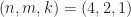
So for BPSK, we need only perform a squaring operation, an FFT, a magnitude operation, and a maximization to find an estimate of $2f_0$ . The accuracy will be limited by the resolution of the FFT, which is approximately equal to the reciprocal of the duration of the processed data block.

To quantify the performance of a basic second-order carrier-offset estimator, I performed Monte Carlo simulations using BPSK with square-root raised-cosine pulses and independent and identically distributed bits for a variety of inband SNRs and block lengths $T$ . For each combination of inband SNR and $T$ , I simulate $1000$ BPSK signals with random carrier phase, symbol-clock phase, carrier frequency offset, and bits. The carrier frequency offset is a uniform random variable on the interval $[-0.051, 0.051]$ in normalized-frequency units. The bit rate is $1/10$ . The carrier offset estimator performance is characterized by the normalized root-mean-squared error (NRMSE), where the RMSE is divided by the FFT bin width $1/T.$ So an NRMSE value of $0.1$ means the RMSE is one-tenth of the reciprocal of the data length.

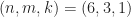
The same method can be applied to the fourth-order lag product with no conjugated factors, leading to a direct estimate of the quadrupled carrier offset $4 f_0$ .

Here are some results for an excess bandwidth of $35$ % and orders $n=2$ and $4:$

Figure 3. Error performance for carrier synchronization using the second-order lag product with no conjugations ( $(n,m,k) = (2, 0, 0)$ ). The error measure is the square-root mean-squared error, which decreases as the processing block size $T$ increases. The signal is square-root raised-cosine BPSK with roll-off parameter 0.35.

Figure 3. Error performance for carrier synchronization using the second-order lag product with no conjugations ( $(n,m,k) = (2, 0, 0)$ ). The error measure is the square-root mean-squared error, which decreases as the processing block size $T$ increases. The signal is square-root raised-cosine BPSK with roll-off parameter 0.35.

Figure 4. Error performance for carrier synchronization using the second-order lag product with no conjugations ( $(n,m,k) = (2, 0, 0)$ ). The error measure is the normalized square-root mean-squared error, which is the RMSE of Figure 3 divided by the FFT bin width $1/T$ . Here we see that the normalized RMSE is constant–the error as a fraction of the FFT width is the same for the various block lengths $T$ . The signal is square-root raised-cosine BPSK with roll-off parameter 0.35.

Figure 5. Error performance for carrier synchronization using the fourth-order lag product with no conjugations ( $(n,m,k) = (4, 0, 0)$ ). The error measure is the square-root mean-squared error, which decreases as the processing block size $T$ increases. The signal is square-root raised-cosine BPSK with roll-off parameter 0.35.

Figure 5. Error performance for carrier synchronization using the fourth-order lag product with no conjugations ( $(n,m,k) = (4, 0, 0)$ ). The error measure is the square-root mean-squared error, which decreases as the processing block size $T$ increases. The signal is square-root raised-cosine BPSK with roll-off parameter 0.35.

nrmse_cfo_4_0_ebw_0.35_BPSK — Figure 6. Error performance for carrier synchronization using the fourth-order lag product with no conjugations ( $(n,m,k) = (4, 0, 0)$ ). The error measure is the normalized square-root mean-squared error, which is the RMSE of Figure 3 divided by the FFT bin width $1/T$ . Here we see that the normalized RMSE is constant–the error as a fraction of the FFT width is the same for the various block lengths $T$ . The signal is square-root raised-cosine BPSK with roll-off parameter 0.35.

And here are the corresponding results for a much smaller excess bandwidth of $5$ %:

rmse_cfo_2_0_ebw_0.05_BPSK — Figure 7. A repeat of the simulation with results in Figure 3 with the sole difference that the BPSK signal has roll-off parameter of 0.05 instead of 0.35.

nrmse_cfo_2_0_ebw_0.05_BPSK — Figure 8. A repeat of the simulation with results in Figure 4 with the sole difference that the BPSK signal has roll-off parameter of 0.05 instead of 0.35.

rmse_cfo_4_0_ebw_0.05_BPSK — Figure 9. A repeat of the simulation with results in Figure 5 with the sole difference that the BPSK signal has roll-off parameter of 0.05 instead of 0.35.

nrmse_cfo_4_0_ebw_0.05_BPSK — Figure 10. A repeat of the simulation with results in Figure 6 with the sole difference that the BPSK signal has roll-off parameter of 0.05 instead of 0.35.

QPSK/QAM: Must use at Least Fourth-Order Statistics for Carrier Offset Estimation

For QPSK and the large-alphabet QAM/PSK signals, the second-order conjugate spectral correlation function is zero, so there is no way to use a second-order moment to obtain a high-resolution estimate of the doubled carrier as we did for BPSK. Instead, for the QAM signals (but not the large-alphabet PSK signals) we can use the fourth-order cyclic moment because it is non-zero for $m=0$ conjugated factors, leading to a set of fourth-order cycle frequencies that take the form

$\displaystyle \alpha(4, 0, k) = 4f_0 + k/T_0 \hfill (15)$

In particular, the sine-wave component in the $(n,m) = (4,0)$ temporal moment with harmonic $k=0$ has the largest magnitude. So the carrier-offset estimation algorithm is nearly identical to that for BPSK, but instead of looking for a peak in the FFT of $x^2(t)$ , we look for a peak in $x^4(t)$ . Here are some typical results, and also the results for applying the BPSK $n=2$ algorithm, fruitlessly, to QPSK:

rmse_cfo_2_0_ebw_0.35_QPSK — Figure 11. Carrier-frequency offset estimation for QPSK using the second-order lag product ( $(n,m,k) = (2, 0, 0)$ ). Although this method is efficacious for BPSK, it fails for QPSK because QPSK does not exhibit conjugate second-order cyclostationarity. The square-root raised-cosine roll-off parameter is 0.35.

nrmse_cfo_2_0_ebw_0.35_QPSK — Figure 12. Normalized CFO error performance for QPSK and second-order processing as in Figure 11. Here the signal does not exhibit conjugate cyclostationarity, and so carrier-frequency offset estimation fails. The error is normalized here by the width of an FFT bin, which is equal to $1/T$ . The square-root raised-cosine roll-off parameter is 0.35.

Figure 12. Normalized CFO error performance for QPSK and second-order processing as in Figure 11. Here the signal does not exhibit conjugate cyclostationarity, and so carrier-frequency offset estimation fails. The error is normalized here by the width of an FFT bin, which is equal to $1/T$ . The square-root raised-cosine roll-off parameter is 0.35.

rmse_cfo_4_0_ebw_0.35_QPSK — Figure 13. Carrier-frequency offset estimation for QPSK using the fourth-order lag product ( $(n,m,k) = (4, 0, 0)$ ). The square-root raised-cosine roll-off parameter is 0.35.

nrmse_cfo_4_0_ebw_0.35_QPSK — Figure 14. Normalized RMSE for the experiment with RMSE shown in Figure 13.

rmse_cfo_2_0_ebw_0.05_QPSK — Figure 15. A repeat of the QPSK experiment with results shown in Figure 11 with the sole difference that the square-root raised-cosine pulse roll-off is changed from 0.35 to 0.05. Since the QPSK signal does not exhibit conjugate cyclostationarity, this second-order method fails.

nrmse_cfo_2_0_ebw_0.05_QPSK — Figure 16. Normalized RMSE performance for the experiment with results in Figure 15.

rmse_cfo_4_0_ebw_0.05_QPSK — Figure 17. A repeat of the QPSK experiment with results shown in Figure 13 with the sole difference that the square-root raised-cosine pulse roll-off is changed from 0.35 to 0.05.

nrmse_cfo_4_0_ebw_0.05_QPSK — Figure 18. Normalized RMSE performance for the experiment with RMSE results shown in Figure 17. The RMSE is normalized by the width of an FFT bin, which is $1/T$ .

Figure 18. Normalized RMSE performance for the experiment with RMSE results shown in Figure 17. The RMSE is normalized by the width of an FFT bin, which is $1/T$ .

Symbol-Clock-Phase Synchronization using Cyclic Moment Functions

To obtain an estimate of the symbol-clock phase, which means determining the relative modulo- $T_0$ delay between an arbitrary reference clock and the clock (timing) of the incoming signal, we can make use of the $(n,m) = (n,n/2)$ cyclic moments, which are sensitive to delay. That is, suppose some signal $s(t)$ has second-order cyclic moment (equivalently, cyclic cumulant for signals possessing no additive sine waves) $R_s^\alpha(\tau;2,1)$ . Then the cyclic moment for $s(t-D)$ is given by $R_s^\alpha(\tau;2,1) e^{-i2\pi \alpha D}$ . If $R_s^\alpha(\tau; 2, 1)$ is real-valued and positive, then we can find the delay $D$ by examining the phase of the cyclic moment estimate. In the following examples, I apply this very simple synchronization method to a BPSK signal with raised-cosine pulses (that is, to the signal after match-filtering has been applied which converts square-root raised-cosine pulses to raised-cosine pulses).

Unlike the case of carrier-offset estimation, the various PSK and QAM signals all possess at least one non-conjugate $(n, m) = (2, 1)$ cycle frequency (the symbol rate), and so we aren’t forced into use of higher-order cyclic moments or cumulants. However, just for fun I’m also showing some results for $(n,m) = (4,2)$ and $(n,m) = (6,3)$ . The root mean-squared error estimates are normalized by the signal’s symbol interval ( $10$ samples).

sym_clock_phase_rmse_nyq_2_1 — Figure 19. Normalized RMSE for a symbol-clock-phase estimate using the non-conjugate second-order cyclic autocorrelation function. Here the signal is BPSK with roll-off of 0.35.

sym_clock_phase_nyq_2_1_copy — Figure 20. Symbol-clock-phase estimates versus the true symbol-clock phase for BPSK with roll-off of 0.35. These results correspond to the experiment with RMSE results shown in Figure 19.

sym_clock_phase_rmse_nyq_4_2 — Figure 21. Normalized RMSE for a symbol-clock-phase estimate using fourth-order cyclic-moment functions with $(n,m,k) = (4,2,1)$ . Here the signal is BPSK with roll-off of 0.35.

Figure 21. Normalized RMSE for a symbol-clock-phase estimate using fourth-order cyclic-moment functions with $(n,m,k) = (4,2,1)$ . Here the signal is BPSK with roll-off of 0.35.

sym_clock_phase_nyq_4_2_copy — Figure 22. Symbol-clock-phase estimates versus the true symbol-clock phase for BPSK with roll-off of 0.35. These results correspond to the experiment with RMSE results shown in Figure 21.

sym_clock_phase_rmse_nyq_6_3 — Fgiure 23. Normalized RMSE for a symbol-clock-phase estimate using fourth-order cyclic-moment functions with $(n,m,k) = (6,3,1)$ . Here the signal is BPSK with roll-off of 0.35.

Fgiure 23. Normalized RMSE for a symbol-clock-phase estimate using fourth-order cyclic-moment functions with $(n,m,k) = (6,3,1)$ . Here the signal is BPSK with roll-off of 0.35.

sym_clock_phase_nyq_6_3_copy — Fgiure 24. Symbol-clock-phase estimates versus the true symbol-clock phase for BPSK with roll-off of 0.35. These results correspond to the experiment with RMSE results shown in Figure 23.

Joint Symbol-Clock and Carrier-Phase Estimation using Cyclic Cumulants

We know that we can estimate the cyclic cumulants for PSK and QAM signals without any knowledge of the synchronization phase parameters–we just need to know the cycle frequencies and the basic modulation type. That means knowledge of the carrier offset $f_0$ and the symbol rate $1/T_0$ . We have those after the carrier-offset synchronization step.

Focusing on the case of cyclic cumulants with delay vectors at the origin, $\boldsymbol{\tau} = \boldsymbol{0}$ , the end result is a matrix of complex-valued cyclic-estimates for a set of $(n, m, k)$ triplets. Each of these values depends on some subset of the synchronization parameters $(t_0, \phi_0)$ . A potentially better performing synchronization method would be to perform a least-squares fit between this matrix and the ideal matrix for the signal type under study. This would result in joint estimation of $(t_0, \phi_0)$ by using multiple orders of cyclic cumulants. An extension would consider multiple such cyclic-cumulant matrices for different non-zero values of the delay vector $\boldsymbol{\tau}$ . I’ll leave this for a future effort. If you pursue it, let me know in the comments!

Author: Chad Spooner

I'm a signal processing researcher specializing in cyclostationary signal processing (CSP) for communication signals. I hope to use this blog to help others with their cyclo-projects and to learn more about how CSP is being used and extended worldwide. View all posts by Chad Spooner

5 thoughts on “Simple Synchronization Using CSP”

MS says:

May 1, 2019 at 11:31 am

Great post! I’m wondering what was the cause of the bump in the RMSE plot for QPSK with EBW = 0.35 using (4, 0) at 13 dB.

Also, what happens if the center frequency is greater than 0.25 so that it wraps around when it is doubled? How would you resolve that ambiguity? Thanks!

1. Chad Spooner says:
  
  May 1, 2019 at 2:04 pm
  
  Thanks MS. Looking back at the data I generated, it looks like that bump was caused by a rather large outlier. True CFO was $-0.04675$ and the estimate was $-0.0217285$ . But I don’t know why that happened…
  
  For the $(2,0)$ algorithm, if the CFO is allowed to be so big, you might first do a simple spectral analysis to determine the centroid of the spectrum. It should be near the CFO, which is greater than $0.25$ for the case you describe. Then the doubled carrier will be estimated as somewhere just greater than $-0.5$ due to wrapping. A CFO just greater than $-0.25$ would also give rise to the $(2,0)$ tone just greater than $-0.5$ . But we can use the centroid to rule out that case. In other words, the CFOs of $0.26$ and $-0.24$ would both give rise to the detected doubled carrier of $-0.48$ , but the centroid of the spectrum can be used to decide between the positive and negative CFO, removing the ambiguity.
  
  I suppose for the $(4,0)$ algorithm, we’d need to do the same sort of thing, but the ambiguity arises for CFOs greater than $0.125$ , not $0.25$ , because it is the quadrupled carrier offset that we are detecting.
  
  Agree?
  
MS says:

May 6, 2019 at 6:22 am

Yes, that makes sense. Though I would imagine it is more difficult with the quadrupled CFO because now you have to look at the possibility of wrapping twice. Thanks!

Andy says:

October 9, 2019 at 7:50 pm

Hi, Dr.Spooner
I am trying to use cyclic moment to blind estimate signal carrier frequency. For example, I use C(4,0) to estimate QPSK carrier frequency. I firstly create a cyclic frequency vector, which include 4*fc value,
then I repeat step (1) – (4) to process each alpha(i)

1) A(t) = s(t).^4, where s(t) = a(t+tau)*exp(j 2pi fc t + theta);
2) B(t) = A(t)*exp(-j2pi* alpha(i)t)
3) repeat step 1) and 2) a few times to get average value of B(t).
4) C(i) = sum( averaged B(t) )

5) Plot Figure, alpha vs C(i), find peak value, which should be located at alpha = 4*fc.

I try a few tests to verify the results. However, a few test is working. So, do I miss anything
in my processing steps?

Thanks.
Andy

1. Chad Spooner says:
  
  October 10, 2019 at 6:09 am
  
  Please review the last section of the post on higher-order cyclic moments and cumulants.