At long last, I am picking up the modulation-recognition (MR) topic again. My plan is to describe the core MR algorithm I’ve developed using cyclic cumulants in this post, and then in a third and final post present some performance results using simulated and captured signals.
Recap of Part I Post
The Part-I post introduced the basic MR problem statement, provided four distinct important problem variations, and discussed the problem aspects that render the problem a perennial one.
The four variations are summarized next.
Radio-Frequency Scene Analysis. The most general version of the problem, as described in my introductory post and my wicked-problem post. For an arbitrary RF scene, detect, characterize, and classify all signals in the scene regardless of their durations, bandwidths, signal-to-interference-and-noise ratios (SINRs), types, and parameters. The cocktail-party problem for radios ™.
Conventional Modulation Classification. The least general version of the problem involves determining the type of a single signal in noise, with moderate-to-high SNR, that is at complex baseband or very close to it. This is the problem considered by most modulation-classification papers of the past four decades, including some of mine.
Cognitive-Radio Modulation Classification. In a modern twist on the problem, cognitive-radio classification involves quickly determining the type of a signal in each of a number of assigned frequency channels used by two kinds of users: Primary and Secondary. The Primary users are the licensed users, and they have right-of-way access to the channels. The Secondary users are non-licensed opportunistic users, attempting to make use of the channels while the Primary users are not. Secondaries must be able to determine what kind of signal is occupying a channel, even if the perceived inband SNR of that occupant is low.
Cochannel Modulation Classification. A difficult version of the problem occurs when two or more signals in the scene can be both contemporaneous and spectrally overlapping. This is called the cochannel signal condition. When the two signals have comparable power, then they each experience a signal-to-interference-and-noise ratio (SINR) of less than zero decibels. So typically the cochannel condition implies low SNR. Moreover, for feature-based classifiers, the features must be signal-selective to be effective, and for trained classifiers, such as trained convolutional neural networks, the training set needs to include all expected (or possible, depending on your biases) combinations of the signals, leading to a combinatorial explosion in the size of the training and testing datasets.
In the Part-I post I assert that the MR problem has not been definitively solved because of the large number of problem dimensions, including catalog size, SNR, cochannel complications, data-record length, sampling bandwidth, desire for real-time operation, and the amount and type of available prior information. I elaborated on this in my speculation that the MR problem is a wicked problem. I also discuss commonly used MR performance measures such as the confusion matrix for decision labels and square-root mean-squared error (RMSE) for parameter estimates. I then describe the major classes of solution approaches, including decision-theoretic, feature-based, and machine-learning. Finally, I present simulated examples that show exactly why various features fail in some important real-world situations.
In this post, I’ll describe my mathematical approach to modulation recognition (decision-theoretic leading to a final principled feature-based algorithm). In Part III, I’ll illustrate the approach with numerical examples.
Algorithm Approach
The mathematical approach to the MR problem is sketched in the companion papers My Papers [26,28], and has roots in a less well-motivated approach I took in My Papers [25]. The remainder of this section, and the section on algorithm development, is an explication of [25,26,28] without the heavy constraint of publication page limits.
Key Background Ideas
Hypothesis Testing
A core idea is that of hypothesis testing. When confronted with a data record containing a single signal with unknown type and parameters, we can imagine forming a sequence of hypotheses (proposed explanation) about that signal. On the first hypothesis, the signal is a BPSK signal. On the second, it is a QPSK signal. On the third, it is an OFDM signal. You can imagine going on like this for some time, leading to a set of, say, 
The formation of hypotheses can be quite simple, as in the binary hypothesis testing problem (BHTP). In the BHTP, there are only two hypotheses. A typical example is hypothesis zero (called 

Many MR situations are not simple, and this leads to the consideration of more complex sets of hypotheses. For example, the first hypothesis could be Type-A Signal is Present and the second could be Type-A Signal is Present with Cochannel Type-B Signal. If there are, say, 

hypotheses. If you have 

Complete Probabilistic Characterizations
We’ll have to carefully consider which hypotheses we include in an MR problem statement, but the discussion above avoided concrete examples of the contents of an individual hypothesis. We said things similar to ‘on hypothesis seven, the signal is BPSK.’ But what exactly does ‘signal is BPSK’ mean here, mathematically? This goes to the heart of my musings on BPSKness in several CSP Blog posts, such as All BPSK Signals and Is RFSA a Wicked Problem?
When we say that on the seventh hypothesis, the data is composed of BPSK plus noise, what does that mean? Here are some possibilities:
- The inphase component of the data (real part) has a graph (plot of the amplitude versus time) that is consistent with that of a BPSK signal with particular values of the pulse-shaping function, bit rate, carrier frequency offset, and allowable transmitted bit sequences.
- The estimated power spectral density is consistent with that of the power spectral density of a BPSK signal with particular parameter values. If you subtract the power-spectrum estimate from the theoretical power spectrum, and summed the absolute value of the resulting difference, the number would be small compared to the energy in the power spectra.
- The set of detectable second-order cycle frequencies for the signal in the data conforms to the pattern of second-order cycle frequencies for a BPSK signal with modern modulation-efficient pulses, such as square-root raised-cosine pulses. The non-conjugate pattern is a single non-zero cycle frequency
. The conjugate pattern is a triplet of cycle frequencies
with
and
.
But, what is the optimal way to form the hypothesis? What is the complete description of BPSKness? If we can capture the full description of what it means for a data sequence or a continuous voltage record to correspond to BPSK–and only to BPSK–then that description would be a good one to use in hypothesis formulation.
Are any of the three alternatives above complete descriptions, in some relevant sense, of BPSKness? Let’s discuss (remember, no page limits here!).
For the first description alternative, we can conceive of a table containing all possible inphase sampled-data or continuous-time functions that correspond to an instance of the BPSK signal in question. That is, fix the bit rate, carrier frequency offset, carrier phase, symbol clock phase, pulse-shaping function, and power (amplitude), and create a table entry for each possible sequence of transmitted bits. We could then do that for all combinations of bit rate, carrier frequency offset, carrier phase, symbol-clock phase, pulse-shaping function, and power. This leads to a very large table–infinite if we take seriously all possible values of, say, the carrier phase (which is an uncountably infinite set because it is a real number).
In the end, we have a table with infinite rows each containing a finite-length complex-valued sequence or function of time. Here, we can formulate a hypothesis for BPSK such as On Hypothesis Seven, the Signal in the Given Data Appears in the BPSK Table. How to make use of this kind of hypothesis, provided we actually have the table? We could form the difference between the data and each row of the table and retain the index of the row for which the sum of the absolute error is minimum. Then repeat that for similar tables for other modulations of interest (you can see the infinities stacking up here I hope). Finally, choose as the modulation-type decision the one corresponding to the minimum table error. For this to be good, we’d have to ensure that the tables for different signal types don’t have significant numbers of identical entries. (Ponder the question of whether a table for QPSK and a table for BPSK will have any identical entries.)
Alternative one isn’t practical–we can’t make these ideal tables and trying to make approximations will also be difficult due to combinatorial explosion. This idea of BPSKness as a giant list of voltage trajectories does bring to mind modern approaches to MR that attempt to create very large I/Q training datasets, which are nothing more than truncated versions of the tables I’ve described. But we have seen over the past five years where that gets us.
The second description alternative is to describe the essential nature of the signal in terms of its power spectrum. Does the estimated power spectrum for the input data match, in some suitable numerical sense, a stored ideal (theoretical) power spectrum for one of the signals of interest? A problem with this alternative is that the power spectrum is not unique for many sets of signal types of interest. I’ve belabored this in other contexts, and it is easily seen to be true. For example, all unit-power PSK and QAM signals with balanced constellations, identical pulse-shaping functions, and independent and identically distributed symbol sequences have identical power spectra.
The third alternative above involves the pattern of second-order cycle frequencies for a signal. In this description, BPSKness involves two small sets of real numbers together with their differences and the relation between the elements of the two sets. If we consider three different signal types: BPSK, QPSK, and AM-DSB, and denote the symbol rate of the PSK signals as 

BPSK:

QPSK:

AM-DSB:

The three sets (second-order cycle-frequency patterns) are highly distinct, which is good for MR. But the flaw in this signalness description is similar to the flaw for the second alternative description that used the power spectrum: A large number of distinct signal types of interest also possess the same cycle-frequency pattern as QPSK. Examples include 8QAM, 16QAM, 64QAM, 
So a big obstacle in the way of setting up a multiple-hypothesis MR problem is how to describe the hypotheses such that each hypothesis captures something unique about the associated signal. And at the same time, avoiding descriptions that are infinite, like the tables above. Some plausible descriptions end up forming undesirable equivalence classes–multiple distinct signals will have identical descriptions in their hypotheses.
But we know that, for instance, QPSK and 16QAM are distinct signal types even if their PSD-based descriptions form an equivalence class. Or do we? Why do we think they are distinct? The question becomes: What does a signal label mean? If all the 16QAM signals are crammed into a box labeled 16QAM, how do we construct the contents of that box? Exactly how do we do that?
I draw your attention back to alternative description one, the infinite table of I/Q trajectories. We’ve seen that before! In the context of random processes, it is the ensemble. And we have a way of generating the entries in the table–the elements of the ensemble–using mathematics. We can write an expression that covers all of the uncountable infinity of ensemble elements; that expression is the ensemble generator. For 16QAM, it is

where 

Most generally, a random process is completely specified by the collection of all possible 

If we wish, we can add more random variables to this process. For example, we can introduce a propagation-channel model such as the discrete multipath channel. For every ensemble element generated by (2), we’d have another uncountable infinity of new ensemble elements, each produced by applying a randomly chosen channel to the chosen element.
So we do have one answer to the question of what constitutes BPSKness: An infinite set of multidimensional (joint) probability density functions. Once those are specified, we can create a random process that will produce all BPSK signals conforming to the underlying random-variable distributions, which is an uncountably infinite set.
The final step in creating hypothesis descriptions is to realize that the set of all possible joint probability density functions for the random process can be expressed in terms of all possible
- The ensemble: A table with an uncountable infinity of rows, each corresponding to one instance of the signal, which means a sample path of the signal’s random-process characterization.
- All joint probability density functions for sets like
- All
.
- All

Likelihood
Consider a random variable 


When this ratio is greater than one, the interpretation is that the observed data (
![\displaystyle \mathcal{L}_X(x) = \ln \left[ \gamma_X(x) \right] \hfill (4)](https://s0.wp.com/latex.php?latex=%5Cdisplaystyle+%5Cmathcal%7BL%7D_X%28x%29+%3D+%5Cln+%5Cleft%5B+%5Cgamma_X%28x%29+%5Cright%5D+%5Chfill+%284%29&bg=ffffff&fg=1a1a1a&s=0&c=20201002)
Suppose the random variable 


A maximum-likelihood decision would then compute each of the likelihoods and choose the hypothesis corresponding to the maximum of those likelihoods.
Problem Statement Evolution
The goal is now to craft a problem statement that captures the modulation-recognition problem and that is mathematically tractable. We also want the problem statement to be as general as possible, so that it is applicable to a large set of modulated signals. To achieve this goal, we present a sequence of problem statements. At first, the problem statements will be equivalent, but eventually we will introduce variations or approximations that result in problem statements that are tractable, and that are not equivalent to the most general problems from the beginning of the sequence.
We want to process some sampled data and decide if that data contains one of 


On the 

For each signal type 
Now let’s consider some label 


which we read as the signal
Problem One
Let’s consider the multiple hypothesis problem given by

for 


Although it is possible to know 
For an arbitrary probability density function, say

that depends on some vector of random variables 

Moreover, the characteristic function itself is a Taylor series involving the moment functions for the sets 

where the
![\displaystyle M_s(t, \boldsymbol{\tau};n) = E\left[ \prod_{j=1}^n s(t+\tau_j) \right]. \hfill (11)](https://s0.wp.com/latex.php?latex=%5Cdisplaystyle+M_s%28t%2C+%5Cboldsymbol%7B%5Ctau%7D%3Bn%29+%3D+E%5Cleft%5B+%5Cprod_%7Bj%3D1%7D%5En+s%28t%2B%5Ctau_j%29+%5Cright%5D.+%5Chfill+%2811%29&bg=ffffff&fg=1a1a1a&s=0&c=20201002)
All the possible moments are found in the multidimensional Taylor-series expansion of the characteristic function. For example, the 

where

is given by the coefficient in the series that corresponds to the term

The point here is that the characteristic functions are completely specified by the set of all possible 
Let’s use some compact notation to try to capture these ideas, which will be critical for our succession of hypotheses-laden problem formulations. Let the symbol 


Saying that a signal is characterized by an infinite set of probability density functions is equivalent to saying that the signal is characterized by an infinite set of
Finally, we make the connection to cumulants. As we saw in the SPTK post on the characteristic function, the natural logarithm of the characteristic function has a series representation in which the coefficients of the various orders of the frequency variables are the cumulants. That is, in the notation we’re using here,

So if you knew all the cumulants, you could construct the logarithm of the characteristic function, and if you know the logarithm of the characteristic function, you can use exponentiation to obtain the characteristic function itself, and if you know the characteristic function, you know the probability density functions. Let’s denote the infinite set of cumulants by 

I emphasize “equivalencies” here–this is not approximately true, it is exactly true. We can now formulate a second problem.
Problem Two
The original problem (7), posed in terms of the infinite set of joint probability density functions 


On the
Problem Three
The problems (7) and (17) are equivalent to a problem posed in terms of an infinite set of cumulant functions 

We can also pose problems in terms of the distribution, moments, or cumulants of the data itself, rather than just for the signal component of the data. Let’s use the notation 


Problem Four

Problem Five

Problem Six

Problems Four, Five, and Six are actually more general than the previous problems because they also include the full probability structure of the noise
We would now like to develop a problem statement that deals with measurable quantities and one with a solution that can be implemented (in software) for a catalog
Elements of 

where 


In (22), the symbol 


Problem Seven

Here we are saying that on the 
As an aside, we can imagine at this point extending Problem Seven to include cochannel signals. We could have a matrix of hypotheses 


Problem Seven gets us closer to a set of hypotheses that involve measured quantities, but isn’t quite there yet, since the specified cumulants are the theoretical cumulants, and so require an infinite ensemble or an infinite-duration signal to average over.
The cumulants can be estimated directly from the data given knowledge of their variation with 
There is a serious dimensionality problem remaining regarding the lag vector 
For the RF communication signals of typical interest to RF scene analysis and modulation recognition, the cumulants are periodically or polyperiodically time-variant, and so we have the Fourier-series representation encountered in the cyclic cumulant post,

where 
We note the equivalence of the time-varying cumulant for signal type

Problem Eight
In this next problem formulation, the hypotheses relate to sets of cyclic cumulants rather than to sets of time-varying cumulants, which eliminates the time variable

for 


So far we have not sacrificed any optimality since the information exploited in Problem Eight is identical to that exploited in Problem One, and in both cases the information consists of the complete (exhaustive) probabilistic description of the involved signal types.
However, the dimensionality of the involved quantities is very large for 
We have two basic choices for dimensionality reduction: restrict the order
Problem Nine
The modification consists of deleting (neglecting) the cyclic cumulant that corresponds to signal power, which means the cyclic cumulant for 


for 
We have left off any mention of the cyclic cumulants for the white Gaussian noise process

We thereby avoid the “second-order stationary” probabilistic parameter but also lose optimality, and we gain sweet simplicity. Moreover, a case of great practical interest corresponds to 
Another good reason for leaving the autocorrelation out of the hypotheses is that when we generalize the hypotheses to the case of cochannel signals, that parameter reflects all of the cochannel signals, not just the 
Problem Ten: The Order-Reduced Classifier
A major simplification of Problem Nine is to severely restrict the order

for 


Problem Eleven
The set of hypotheses (30) suggests the following practical problem, where the limit probabilistic parameter for the received data is replaced by a noisy estimate,

for 
Problem Eleven is recognized as a known-signal-in-noise problem (a matched-filtering problem). The problem is easy when the cycle frequencies for the different hypotheses are disjoint–that is, when the signals all have different cycle frequencies. We focus on the harder problem, which is of substantial practical interest, where all the signals have the same cycle frequency sets,


Problem Eleven is then simplified to

for 
Further simplifications are possible. Note that the information in a single cyclic cumulant function requires only 


where the 
![\displaystyle \boldsymbol{u} = \left[ \tau_1-\tau_n, \tau_2-\tau_n, \ldots, \tau_{n-1}-\tau_n\right]. \hfill (33)](https://s0.wp.com/latex.php?latex=%5Cdisplaystyle+%5Cboldsymbol%7Bu%7D+%3D+%5Cleft%5B+%5Ctau_1-%5Ctau_n%2C+%5Ctau_2-%5Ctau_n%2C+%5Cldots%2C+%5Ctau_%7Bn-1%7D-%5Ctau_n%5Cright%5D.+%5Chfill+%2833%29&bg=ffffff&fg=1a1a1a&s=0&c=20201002)
More generally, we simply use the 
Let’s name the second-order cycle frequencies 


for 


Finally, we make the simplifying assumption that the noise 

Solution to Problem Eleven: The ORC
If the amplitude 


For each 


and variance 
![[-T, T]](https://s0.wp.com/latex.php?latex=%5B-T%2C+T%5D&bg=ffffff&fg=1a1a1a&s=0&c=20201002)


![\displaystyle \hat{\bar{\boldsymbol{C}}} = \left[ \hat{\bar{C}}_{re} \ \ \hat{\bar{C}}_{im} \right]](https://s0.wp.com/latex.php?latex=%5Cdisplaystyle+%5Chat%7B%5Cbar%7B%5Cboldsymbol%7BC%7D%7D%7D+%3D%C2%A0+%5Cleft%5B+%5Chat%7B%5Cbar%7BC%7D%7D_%7Bre%7D+%5C+%5C+%5Chat%7B%5Cbar%7BC%7D%7D_%7Bim%7D+%5Cright%5D&bg=ffffff&fg=1a1a1a&s=0&c=20201002)
where
![\displaystyle \hat{\bar{C}}_{re} = \Re \left[ \underbrace{\hat{\bar{C}}_x^{\gamma_1} (-T, 2) \cdots \hat{\bar{C}}_x^{\gamma_1} (T, 2)}_{\gamma_1} \cdots \underbrace{\hat{\bar{C}}_x^{\gamma_{N_2}} (-T, 2) \cdots \hat{\bar{C}}_x^{\gamma_{N_2}} (T, 2)}_{\gamma_{N_2}} \right] \hfill (36)](https://s0.wp.com/latex.php?latex=%5Cdisplaystyle+%5Chat%7B%5Cbar%7BC%7D%7D_%7Bre%7D+%3D+%5CRe+%5Cleft%5B+%5Cunderbrace%7B%5Chat%7B%5Cbar%7BC%7D%7D_x%5E%7B%5Cgamma_1%7D+%28-T%2C+2%29+%5Ccdots+%5Chat%7B%5Cbar%7BC%7D%7D_x%5E%7B%5Cgamma_1%7D+%28T%2C+2%29%7D_%7B%5Cgamma_1%7D+%5Ccdots%C2%A0+%C2%A0+%5Cunderbrace%7B%5Chat%7B%5Cbar%7BC%7D%7D_x%5E%7B%5Cgamma_%7BN_2%7D%7D+%28-T%2C+2%29+%5Ccdots+%5Chat%7B%5Cbar%7BC%7D%7D_x%5E%7B%5Cgamma_%7BN_2%7D%7D+%28T%2C+2%29%7D_%7B%5Cgamma_%7BN_2%7D%7D+%5Cright%5D+%5Chfill+%2836%29&bg=ffffff&fg=1a1a1a&s=0&c=20201002)
![\displaystyle \hat{\bar{C}}_{im} = \Im \left[ \underbrace{\hat{\bar{C}}_x^{\gamma_1} (-T, 2) \cdots \hat{\bar{C}}_x^{\gamma_1} (T, 2)}_{\gamma_1} \cdots \underbrace{\hat{\bar{C}}_x^{\gamma_{N_2}} (-T, 2) \cdots \hat{\bar{C}}_x^{\gamma_{N_2}} (T, 2)}_{\gamma_{N_2}}\right] \hfill (37)](https://s0.wp.com/latex.php?latex=%5Cdisplaystyle+%5Chat%7B%5Cbar%7BC%7D%7D_%7Bim%7D+%3D+%5CIm+%5Cleft%5B+%5Cunderbrace%7B%5Chat%7B%5Cbar%7BC%7D%7D_x%5E%7B%5Cgamma_1%7D+%28-T%2C+2%29+%5Ccdots+%5Chat%7B%5Cbar%7BC%7D%7D_x%5E%7B%5Cgamma_1%7D+%28T%2C+2%29%7D_%7B%5Cgamma_1%7D+%5Ccdots%C2%A0+%C2%A0+%5Cunderbrace%7B%5Chat%7B%5Cbar%7BC%7D%7D_x%5E%7B%5Cgamma_%7BN_2%7D%7D+%28-T%2C+2%29+%5Ccdots+%5Chat%7B%5Cbar%7BC%7D%7D_x%5E%7B%5Cgamma_%7BN_2%7D%7D+%28T%2C+2%29%7D_%7B%5Cgamma_%7BN_2%7D%7D%5Cright%5D+%5Chfill+%2837%29&bg=ffffff&fg=1a1a1a&s=0&c=20201002)
Through this sequence of definitions, approximations, and assumptions (some quite probably questionable), we arrive at a vector 
![\displaystyle \hat{\bar{C}}_x^{\gamma_j} (k, 2)_r = \Re \left[ \hat{\bar{C}}_x^{\gamma_j} (k, 2) \right] \hfill (38)](https://s0.wp.com/latex.php?latex=%5Cdisplaystyle+%5Chat%7B%5Cbar%7BC%7D%7D_x%5E%7B%5Cgamma_j%7D+%28k%2C+2%29_r+%3D+%5CRe+%5Cleft%5B+%5Chat%7B%5Cbar%7BC%7D%7D_x%5E%7B%5Cgamma_j%7D+%28k%2C+2%29+%5Cright%5D+%5Chfill+%2838%29&bg=ffffff&fg=1a1a1a&s=0&c=20201002)
![\displaystyle \hat{\bar{C}}_x^{\gamma_j} (k, 2)_i = \Im \left[ \hat{\bar{C}}_x^{\gamma_j} (k, 2) \right] \hfill (39)](https://s0.wp.com/latex.php?latex=%5Cdisplaystyle+%5Chat%7B%5Cbar%7BC%7D%7D_x%5E%7B%5Cgamma_j%7D+%28k%2C+2%29_i+%3D+%5CIm+%5Cleft%5B+%5Chat%7B%5Cbar%7BC%7D%7D_x%5E%7B%5Cgamma_j%7D+%28k%2C+2%29+%5Cright%5D+%5Chfill+%2839%29&bg=ffffff&fg=1a1a1a&s=0&c=20201002)
to enable us to write the joint probability density function for the elements of 
![\displaystyle P(\hat{\bar{\boldsymbol{C}}}|H_i) = \prod_{j=1}^{N_2} \left[ \prod_{k=-T}^T \left(\frac{1}{\sqrt{2}\pi (\sigma_\nu^2/2)} \right) e^{\left(-\frac{[\hat{\bar{C}}_x^{\gamma_j}(k,2)_r - E[\hat{\bar{C}}_x^{\gamma_j}(k,2)_r] ]^2}{\sigma_\nu^2}\right)}\right.](https://s0.wp.com/latex.php?latex=%5Cdisplaystyle+P%28%5Chat%7B%5Cbar%7B%5Cboldsymbol%7BC%7D%7D%7D%7CH_i%29+%3D+%5Cprod_%7Bj%3D1%7D%5E%7BN_2%7D+%5Cleft%5B+%5Cprod_%7Bk%3D-T%7D%5ET+%5Cleft%28%5Cfrac%7B1%7D%7B%5Csqrt%7B2%7D%5Cpi+%28%5Csigma_%5Cnu%5E2%2F2%29%7D+%5Cright%29+e%5E%7B%5Cleft%28-%5Cfrac%7B%5B%5Chat%7B%5Cbar%7BC%7D%7D_x%5E%7B%5Cgamma_j%7D%28k%2C2%29_r+-+E%5B%5Chat%7B%5Cbar%7BC%7D%7D_x%5E%7B%5Cgamma_j%7D%28k%2C2%29_r%5D+%5D%5E2%7D%7B%5Csigma_%5Cnu%5E2%7D%5Cright%29%7D%5Cright.+&bg=ffffff&fg=1a1a1a&s=0&c=20201002)
![\displaystyle \times \left. \prod_{l=-T}^T \left(\frac{1}{\sqrt{2}\pi (\sigma_\nu^2/2)} \right) e^{\left(-\frac{[\hat{\bar{C}}_x^{\gamma_j}(l,2)_i - E[\hat{\bar{C}}_x^{\gamma_j}(l,2)_i] ]^2}{\sigma_\nu^2}\right)}\right] \hfill (40)](https://s0.wp.com/latex.php?latex=%5Cdisplaystyle+%5Ctimes+%5Cleft.+%5Cprod_%7Bl%3D-T%7D%5ET+%5Cleft%28%5Cfrac%7B1%7D%7B%5Csqrt%7B2%7D%5Cpi+%28%5Csigma_%5Cnu%5E2%2F2%29%7D+%5Cright%29+e%5E%7B%5Cleft%28-%5Cfrac%7B%5B%5Chat%7B%5Cbar%7BC%7D%7D_x%5E%7B%5Cgamma_j%7D%28l%2C2%29_i+-+E%5B%5Chat%7B%5Cbar%7BC%7D%7D_x%5E%7B%5Cgamma_j%7D%28l%2C2%29_i%5D+%5D%5E2%7D%7B%5Csigma_%5Cnu%5E2%7D%5Cright%29%7D%5Cright%5D+%5Chfill+%2840%29&bg=ffffff&fg=1a1a1a&s=0&c=20201002)
Let’s simplify the notation for the mean values,
![\displaystyle D_{s_i}^{\gamma_j} (\tau, 2)_r = \Re \left[ \hat{a}_i^2 \bar{C}_{s_i}^{\gamma_j} (\tau, 2) e^{-i2\pi \gamma_j \hat{t}_{0,i}} \right] \hfill (41)](https://s0.wp.com/latex.php?latex=%5Cdisplaystyle+D_%7Bs_i%7D%5E%7B%5Cgamma_j%7D+%28%5Ctau%2C+2%29_r+%3D+%5CRe+%5Cleft%5B+%5Chat%7Ba%7D_i%5E2+%5Cbar%7BC%7D_%7Bs_i%7D%5E%7B%5Cgamma_j%7D+%28%5Ctau%2C+2%29+e%5E%7B-i2%5Cpi+%5Cgamma_j+%5Chat%7Bt%7D_%7B0%2Ci%7D%7D+%5Cright%5D+%5Chfill+%2841%29&bg=ffffff&fg=1a1a1a&s=0&c=20201002)
![\displaystyle D_{s_i}^{\gamma_j} (\tau, 2)_i = \Im \left[ \hat{a}_i^2 \bar{C}_{s_i}^{\gamma_j} (\tau, 2) e^{-i2\pi \gamma_j \hat{t}_{0,i}} \right] \hfill (42)](https://s0.wp.com/latex.php?latex=%5Cdisplaystyle+D_%7Bs_i%7D%5E%7B%5Cgamma_j%7D+%28%5Ctau%2C+2%29_i+%3D+%5CIm+%5Cleft%5B+%5Chat%7Ba%7D_i%5E2+%5Cbar%7BC%7D_%7Bs_i%7D%5E%7B%5Cgamma_j%7D+%28%5Ctau%2C+2%29+e%5E%7B-i2%5Cpi+%5Cgamma_j+%5Chat%7Bt%7D_%7B0%2Ci%7D%7D+%5Cright%5D+%5Chfill+%2842%29&bg=ffffff&fg=1a1a1a&s=0&c=20201002)
![\displaystyle P(\hat{\bar{\boldsymbol{C}}}|H_i) = \prod_{j=1}^{N_2} \left[ \prod_{k=-T}^T \left(\frac{1}{\sqrt{2}\pi (\sigma_\nu^2/2)} \right) e^{\left(-\frac{[\hat{\bar{C}}_x^{\gamma_j}(k,2)_r - D_{s_i}^{\gamma_j}(k,2)_r ]^2}{\sigma_\nu^2}\right)}\right.](https://s0.wp.com/latex.php?latex=%5Cdisplaystyle+P%28%5Chat%7B%5Cbar%7B%5Cboldsymbol%7BC%7D%7D%7D%7CH_i%29+%3D+%5Cprod_%7Bj%3D1%7D%5E%7BN_2%7D+%5Cleft%5B+%5Cprod_%7Bk%3D-T%7D%5ET+%5Cleft%28%5Cfrac%7B1%7D%7B%5Csqrt%7B2%7D%5Cpi+%28%5Csigma_%5Cnu%5E2%2F2%29%7D+%5Cright%29+e%5E%7B%5Cleft%28-%5Cfrac%7B%5B%5Chat%7B%5Cbar%7BC%7D%7D_x%5E%7B%5Cgamma_j%7D%28k%2C2%29_r+-+D_%7Bs_i%7D%5E%7B%5Cgamma_j%7D%28k%2C2%29_r+%5D%5E2%7D%7B%5Csigma_%5Cnu%5E2%7D%5Cright%29%7D%5Cright.+&bg=ffffff&fg=1a1a1a&s=0&c=20201002)
![\displaystyle \times \left. \prod_{l=-T}^T \left(\frac{1}{\sqrt{2}\pi (\sigma_\nu^2/2)} \right) e^{\left(-\frac{[\hat{\bar{C}}_x^{\gamma_j}(l,2)_i - D_{s_i}^{\gamma_j}(l,2)_i ]^2}{\sigma_\nu^2}\right)}\right] \hfill (43)](https://s0.wp.com/latex.php?latex=%5Cdisplaystyle+%5Ctimes+%5Cleft.+%5Cprod_%7Bl%3D-T%7D%5ET+%5Cleft%28%5Cfrac%7B1%7D%7B%5Csqrt%7B2%7D%5Cpi+%28%5Csigma_%5Cnu%5E2%2F2%29%7D+%5Cright%29+e%5E%7B%5Cleft%28-%5Cfrac%7B%5B%5Chat%7B%5Cbar%7BC%7D%7D_x%5E%7B%5Cgamma_j%7D%28l%2C2%29_i+-+D_%7Bs_i%7D%5E%7B%5Cgamma_j%7D%28l%2C2%29_i+%5D%5E2%7D%7B%5Csigma_%5Cnu%5E2%7D%5Cright%29%7D%5Cright%5D+%5Chfill+%2843%29&bg=ffffff&fg=1a1a1a&s=0&c=20201002)
Our density function can be slightly simplified to
![\displaystyle P(\hat{\bar{\boldsymbol{C}}}|H_i) =\left(\frac{\sqrt{2}}{\pi (\sigma_\nu^2/2)} \right)^{2N_2(2T_1)} \prod_{j=1}^{N_2} \left[ \prod_{k=-T}^T e^{\left(-\frac{[\hat{\bar{C}}_x^{\gamma_j}(k,2)_r - D_{s_i}^{\gamma_j}(k,2)_r ]^2}{\sigma_\nu^2}\right)}\right.](https://s0.wp.com/latex.php?latex=%5Cdisplaystyle+P%28%5Chat%7B%5Cbar%7B%5Cboldsymbol%7BC%7D%7D%7D%7CH_i%29+%3D%5Cleft%28%5Cfrac%7B%5Csqrt%7B2%7D%7D%7B%5Cpi+%28%5Csigma_%5Cnu%5E2%2F2%29%7D+%5Cright%29%5E%7B2N_2%282T_1%29%7D+%5Cprod_%7Bj%3D1%7D%5E%7BN_2%7D+%5Cleft%5B+%5Cprod_%7Bk%3D-T%7D%5ET%C2%A0+e%5E%7B%5Cleft%28-%5Cfrac%7B%5B%5Chat%7B%5Cbar%7BC%7D%7D_x%5E%7B%5Cgamma_j%7D%28k%2C2%29_r+-+D_%7Bs_i%7D%5E%7B%5Cgamma_j%7D%28k%2C2%29_r+%5D%5E2%7D%7B%5Csigma_%5Cnu%5E2%7D%5Cright%29%7D%5Cright.+&bg=ffffff&fg=1a1a1a&s=0&c=20201002)
![\displaystyle \times \left. e^{\left(-\frac{[\hat{\bar{C}}_x^{\gamma_j}(k,2)_i - D_{s_i}^{\gamma_j}(k,2)_i ]^2}{\sigma_\nu^2}\right)}\right] \hfill (44)](https://s0.wp.com/latex.php?latex=%5Cdisplaystyle+%5Ctimes+%5Cleft.%C2%A0+%C2%A0e%5E%7B%5Cleft%28-%5Cfrac%7B%5B%5Chat%7B%5Cbar%7BC%7D%7D_x%5E%7B%5Cgamma_j%7D%28k%2C2%29_i+-+D_%7Bs_i%7D%5E%7B%5Cgamma_j%7D%28k%2C2%29_i+%5D%5E2%7D%7B%5Csigma_%5Cnu%5E2%7D%5Cright%29%7D%5Cright%5D+%5Chfill+%2844%29&bg=ffffff&fg=1a1a1a&s=0&c=20201002)
We can now compute the logarithm of the density function (which is also a likelihood function), which will simplify finding its extremal values, leading to a method of signal classification. That is, we want to find the index
The logarithm converts the products to sums,

![\displaystyle \left. +2\hat{\bar{C}}_x^{\gamma_j}(k,2)_rD_{s_i}^{\gamma_j}(k,2)_r + 2\hat{\bar{C}}_x^{\gamma_j}(k,2)_i D_{s_i}^{\gamma_j}(k,2)_i \right] \hfill (45)](https://s0.wp.com/latex.php?latex=%5Cdisplaystyle+%5Cleft.+%2B2%5Chat%7B%5Cbar%7BC%7D%7D_x%5E%7B%5Cgamma_j%7D%28k%2C2%29_rD_%7Bs_i%7D%5E%7B%5Cgamma_j%7D%28k%2C2%29_r+%2B+2%5Chat%7B%5Cbar%7BC%7D%7D_x%5E%7B%5Cgamma_j%7D%28k%2C2%29_i+D_%7Bs_i%7D%5E%7B%5Cgamma_j%7D%28k%2C2%29_i+%5Cright%5D+%5Chfill+%2845%29&bg=ffffff&fg=1a1a1a&s=0&c=20201002)

Substituting the definition of 

If we want to maximize the conditional density function over the various signal-type hypotheses indexed by

Discussion
The order-reduced version of our general problem results in a relatively simple distance-based classifier embodied by Equation (48). This classifier compares all cyclic autocorrelation functions in the catalog of known types with the measured cyclic autocorrelation functions obtained from the data at hand. It can work provided no entries of the catalog set

where 
Unfortunately, there are many signals for which the condition (49) does not hold. In particular, all PSK signals with four or more points in their constellation, and where the constellation is doubly symmetric in the complex plane, have identical second-order statistics. This can be referred to as an equivalence class. The signals for which (49) does not hold form a subset of signal types that are equivalent with respect to the lens of second-order limit parameters (time-varying mean and time-varying autocorrelation).
To accurately distinguish between signals that fall into such an equivalence class, we can consider a delay-reduced version of the general problem instead of the order-reduced version (Problem Nine). For this new problem variant, we restrict the range of the 

Problem Twelve
Our hypotheses are now given by

for 


where 
The formulation in (49) can be expressed in terms of the specific cycle frequencies

where 

We next introduce the concept of cumulant warping in which each 


The next Problem Twelve variant is
![\displaystyle H_i: \left[ \bar{C}_x^{\gamma_{i,n}(j)}(\boldsymbol{0};n) \right]^{2/n} = \hat{a}_i^2 \left[ \bar{C}_{s_i}^{\gamma_{i,n}(j)}(\boldsymbol{0}; n) \right]^{2/n} e^{-i4\pi \gamma_{i,n}(j)\hat{t}_{0,i}/n} \hfill (52)](https://s0.wp.com/latex.php?latex=%5Cdisplaystyle+H_i%3A+%5Cleft%5B+%5Cbar%7BC%7D_x%5E%7B%5Cgamma_%7Bi%2Cn%7D%28j%29%7D%28%5Cboldsymbol%7B0%7D%3Bn%29+%5Cright%5D%5E%7B2%2Fn%7D+%3D+%5Chat%7Ba%7D_i%5E2+%5Cleft%5B+%5Cbar%7BC%7D_%7Bs_i%7D%5E%7B%5Cgamma_%7Bi%2Cn%7D%28j%29%7D%28%5Cboldsymbol%7B0%7D%3B+n%29+%5Cright%5D%5E%7B2%2Fn%7D+e%5E%7B-i4%5Cpi+%5Cgamma_%7Bi%2Cn%7D%28j%29%5Chat%7Bt%7D_%7B0%2Ci%7D%2Fn%7D+%5Chfill+%2852%29&bg=ffffff&fg=1a1a1a&s=0&c=20201002)
where
Let’s now (naively) assume that these nonlinearly transformed cyclic cumulants can be estimated with variance independent of both
![\displaystyle H_i: \left[ \hat{\bar{C}}_x^{\gamma_{i,n}(j)} (\boldsymbol{0};n) \right]^{2/n} = \hat{a}_i^2 \left[ \bar{C}_{s_i}^{\gamma_{i,n}(j)} (\boldsymbol{0};n) \right]^{2/n} e^{-i4 \gamma_{i,n}(j) \hat{t}_{0,i}/n} + \nu(\gamma_{i,n}(j), n) \hfill (53)](https://s0.wp.com/latex.php?latex=%5Cdisplaystyle+H_i%3A+%5Cleft%5B+%5Chat%7B%5Cbar%7BC%7D%7D_x%5E%7B%5Cgamma_%7Bi%2Cn%7D%28j%29%7D+%28%5Cboldsymbol%7B0%7D%3Bn%29+%5Cright%5D%5E%7B2%2Fn%7D+%3D+%5Chat%7Ba%7D_i%5E2+%5Cleft%5B+%5Cbar%7BC%7D_%7Bs_i%7D%5E%7B%5Cgamma_%7Bi%2Cn%7D%28j%29%7D+%28%5Cboldsymbol%7B0%7D%3Bn%29+%5Cright%5D%5E%7B2%2Fn%7D+e%5E%7B-i4+%5Cgamma_%7Bi%2Cn%7D%28j%29+%5Chat%7Bt%7D_%7B0%2Ci%7D%2Fn%7D+%2B+%5Cnu%28%5Cgamma_%7Bi%2Cn%7D%28j%29%2C+n%29+%5Chfill+%2853%29&bg=ffffff&fg=1a1a1a&s=0&c=20201002)
where 

For convenience, let’s compact the notation
![\displaystyle \hat{D}_x^{\gamma_{i,n}(j)}(n) = \left[ \hat{C}_x^{\gamma_{i,n}(j)}(\boldsymbol{0};n) \right]^{2/n} \hfill (54)](https://s0.wp.com/latex.php?latex=%5Cdisplaystyle+%5Chat%7BD%7D_x%5E%7B%5Cgamma_%7Bi%2Cn%7D%28j%29%7D%28n%29+%3D+%5Cleft%5B+%5Chat%7BC%7D_x%5E%7B%5Cgamma_%7Bi%2Cn%7D%28j%29%7D%28%5Cboldsymbol%7B0%7D%3Bn%29+%5Cright%5D%5E%7B2%2Fn%7D+%5Chfill+%2854%29&bg=ffffff&fg=1a1a1a&s=0&c=20201002)
![\displaystyle D_{s_i}^{\gamma_{i,n}(j)} (n) = \hat{a}_i^2 \left[ \bar{C}_{s_i}^{\gamma_{i,n}(j)} (\boldsymbol{0};n) \right]^{2/n} e^{-i 4 \pi \gamma_{i,n}(j) \hat{t}_{0,i}/n} \hfill (55)](https://s0.wp.com/latex.php?latex=%5Cdisplaystyle+D_%7Bs_i%7D%5E%7B%5Cgamma_%7Bi%2Cn%7D%28j%29%7D+%28n%29+%3D+%5Chat%7Ba%7D_i%5E2+%5Cleft%5B+%5Cbar%7BC%7D_%7Bs_i%7D%5E%7B%5Cgamma_%7Bi%2Cn%7D%28j%29%7D+%28%5Cboldsymbol%7B0%7D%3Bn%29+%5Cright%5D%5E%7B2%2Fn%7D+e%5E%7B-i+4+%5Cpi+%5Cgamma_%7Bi%2Cn%7D%28j%29+%5Chat%7Bt%7D_%7B0%2Ci%7D%2Fn%7D+%5Chfill+%2855%29&bg=ffffff&fg=1a1a1a&s=0&c=20201002)
Then our final variant of Problem Twelve is simply

where
The interpretation of Problem Twelve is that on the
Solution to Problem Twelve
Since (56) is a form of the known-signal-in-noise problem, we can immediately write the solution,

Or, back substituting for the
![\displaystyle \hat{i} = \mbox{\rm arg} \max_{i \in B} \sum_{n=1}^{N_{max}} \sum_{j=1}^{N_n} \left| \left[ \hat{\bar{C}}_x^{\gamma_{i,n}(j)} (\boldsymbol{0}; n) \right]^{2/n} - \hat{a}_i^2 \left[ C_{s_i}^{\gamma_{i,n}(j)} (\boldsymbol{0}; n) \right]^{2/n} e^{-i 4 \pi \gamma_{i,n}(j) \hat{t}_{0,i} /n} \right|^2 \hfill (58)](https://s0.wp.com/latex.php?latex=%5Cdisplaystyle+%5Chat%7Bi%7D+%3D+%5Cmbox%7B%5Crm+arg%7D+%5Cmax_%7Bi+%5Cin+B%7D+%5Csum_%7Bn%3D1%7D%5E%7BN_%7Bmax%7D%7D+%5Csum_%7Bj%3D1%7D%5E%7BN_n%7D+%5Cleft%7C+%5Cleft%5B+%5Chat%7B%5Cbar%7BC%7D%7D_x%5E%7B%5Cgamma_%7Bi%2Cn%7D%28j%29%7D+%28%5Cboldsymbol%7B0%7D%3B+n%29+%5Cright%5D%5E%7B2%2Fn%7D+-+%5Chat%7Ba%7D_i%5E2+%5Cleft%5B+C_%7Bs_i%7D%5E%7B%5Cgamma_%7Bi%2Cn%7D%28j%29%7D+%28%5Cboldsymbol%7B0%7D%3B+n%29+%5Cright%5D%5E%7B2%2Fn%7D+e%5E%7B-i+4+%5Cpi+%5Cgamma_%7Bi%2Cn%7D%28j%29+%5Chat%7Bt%7D_%7B0%2Ci%7D+%2Fn%7D+%5Cright%7C%5E2+%5Chfill+%2858%29&bg=ffffff&fg=1a1a1a&s=0&c=20201002)
The interpretation of the solution to Problem Twelve is that the best decision index corresponds to the minimum of the sum of squared distances between the signal’s ideal cyclic cumulants and the corresponding measured cyclic cumulants, or what I call cyclic-cumulant matching.
Reverie
That was a lot. And, I am sorry to say, not one figure has yet been placed into this exposition. We ended up with two likelihood-based (decision theoretic) signal classifiers that are each a major simplification of a much more complete and imposing signal classifier. Along the way, we thought hard about how to capture the probabilistic essence of a manmade communication signal. As I say elsewhere on the CSP Blog, what makes a BPSK signal a BPSK signal? What is BPSKness? I opted to pursue a series of problem statements that focused on the notion that a signal’s unique signalness can be completely captured by the infinite set of all of its cumulants.
In this post we are able to take a lot of time, and a lot of words and equations, to get us to a potentially useful algorithm. Now compare what we did here with what I wrote in My Papers [28], which also presents the order-reduced and delay-reduced classifiers. I simply can’t go through all the intermediate steps in a published paper–there is always a severe page limit relative to the writing and equations required by a complicated R&D algorithm-development project.
Extensions
Power-Constrained Classification
The restriction on distinct catalog elements for both the order-reduced and delay-reduced classifiers can be eased if prior information on the signal power is available.
Order-Reduced Classifier with Power Constraint
Since all catalog elements arise from signal models with unit power, the variable 
Suppose, though, that we obtain a hypothesis-independent estimate of 

subject to

We choose the maximum likelihood catalog entry subject to a constraint on the estimated power level; estimated power levels that are too far removed from the independent estimate 
We have increased our tolerance to similar catalog entries for the order-reduced classifier, but it still fails when two catalog entries are actually identical. Such entries would yield identical dependent power levels, rendering the constraint useless to discriminate between them.
Delay-Reduced Classifier with Power Constraint
We can introduce the same constraint to the delay-reduced classifier to accommodate warped cyclic-cumulant catalog entries that are scaled versions of each other,
![\displaystyle \hat{i} = \mbox{\rm arg} \min_{i \in B} \sum_{n=1}^{N_{max}} \sum_{j=1}^{N_n} \left| \left[ \hat{C}_x^{\gamma_{i,n(j)}} (\boldsymbol{0};n) \right]^{2/n} - \hat{a}_i^2 \left[ \hat{C}_{s_i}^{\gamma_{i,n}(j)} (\boldsymbol{0};n) \right]^{2/n} e^{-i4\pi \gamma_{i,n}(j) \hat{t}_{0,i}/n} \right|^2 \hfill (61)](https://s0.wp.com/latex.php?latex=%5Cdisplaystyle+%5Chat%7Bi%7D+%3D+%5Cmbox%7B%5Crm+arg%7D+%5Cmin_%7Bi+%5Cin+B%7D+%5Csum_%7Bn%3D1%7D%5E%7BN_%7Bmax%7D%7D+%5Csum_%7Bj%3D1%7D%5E%7BN_n%7D+%5Cleft%7C+%5Cleft%5B+%5Chat%7BC%7D_x%5E%7B%5Cgamma_%7Bi%2Cn%28j%29%7D%7D+%28%5Cboldsymbol%7B0%7D%3Bn%29+%5Cright%5D%5E%7B2%2Fn%7D+-+%5Chat%7Ba%7D_i%5E2+%5Cleft%5B+%5Chat%7BC%7D_%7Bs_i%7D%5E%7B%5Cgamma_%7Bi%2Cn%7D%28j%29%7D+%28%5Cboldsymbol%7B0%7D%3Bn%29+%5Cright%5D%5E%7B2%2Fn%7D+e%5E%7B-i4%5Cpi+%5Cgamma_%7Bi%2Cn%7D%28j%29+%5Chat%7Bt%7D_%7B0%2Ci%7D%2Fn%7D+%5Cright%7C%5E2+%5Chfill+%2861%29&bg=ffffff&fg=1a1a1a&s=0&c=20201002)
subject to

Discussion
The use of the power constraint in the two derived classifiers might seem strange. Why not simply replace the hypothesis-dependent power estimates
If I give you the sum of two students’ test scores (say, 152), can you tell me the two scores?
Multiple Cochannel Signals
Our cochannel signal model is a simple generalization of our original model (7),

The cochannel model for which the 
We now develop a sequence of hypothesis-testing problems that parallels the previous single-signal development. In this development, we assume the number of signals
In the single-signal case, a hypothesis consisted of the identification of a probability structure for the signal,

We now identify a hypothesis with the selection of a probability structure that incorporates the individual probability structures for each of the

where 
![\displaystyle \boldsymbol{s}(t) = \left[ s_1(t-t_1) \ s_2(t-t_2) \ldots s_M(t-t_M)\right] \hfill (66)](https://s0.wp.com/latex.php?latex=%5Cdisplaystyle+%5Cboldsymbol%7Bs%7D%28t%29+%3D+%5Cleft%5B+s_1%28t-t_1%29+%5C+s_2%28t-t_2%29+%5Cldots+s_M%28t-t_M%29%5Cright%5D+%5Chfill+%2866%29&bg=ffffff&fg=1a1a1a&s=0&c=20201002)
and 
![\displaystyle \boldsymbol{a} = [a_1 \ a_2 \ldots a_M] \hfill (67)](https://s0.wp.com/latex.php?latex=%5Cdisplaystyle+%5Cboldsymbol%7Ba%7D+%3D+%5Ba_1+%5C%C2%A0+a_2+%5Cldots+a_M%5D+%5Chfill+%2867%29&bg=ffffff&fg=1a1a1a&s=0&c=20201002)
and 
We say that 


![\displaystyle \boldsymbol{i} = [i_1 \ i_2 \ldots i_M] \in B^M = \underbrace{B \times B \times \ldots \times B}_{M} \hfill (69)](https://s0.wp.com/latex.php?latex=%5Cdisplaystyle+%5Cboldsymbol%7Bi%7D+%3D+%5Bi_1+%5C+i_2+%5Cldots+i_M%5D+%5Cin+B%5EM+%3D+%5Cunderbrace%7BB+%5Ctimes+B+%5Ctimes+%5Cldots+%5Ctimes+B%7D_%7BM%7D+%5Chfill+%2869%29&bg=ffffff&fg=1a1a1a&s=0&c=20201002)
![\displaystyle \boldsymbol{\mathcal{P}}_{\boldsymbol{i}} = \left[\mathcal{P}_{i_1} \ \mathcal{P}_{i_2} \ldots \mathcal{P}_{i_M} \right] \hfill (70)](https://s0.wp.com/latex.php?latex=%5Cdisplaystyle+%5Cboldsymbol%7B%5Cmathcal%7BP%7D%7D_%7B%5Cboldsymbol%7Bi%7D%7D+%3D+%5Cleft%5B%5Cmathcal%7BP%7D_%7Bi_1%7D+%5C+%5Cmathcal%7BP%7D_%7Bi_2%7D+%5Cldots+%5Cmathcal%7BP%7D_%7Bi_M%7D+%5Cright%5D+%5Chfill+%2870%29&bg=ffffff&fg=1a1a1a&s=0&c=20201002)

Problem Thirteen
Our first cochannel-signal hypothesis is simply

We can form equivalent problem statements using either moments or cumulants,


The cumulant formulation is preferred because the cumulant structure of

Since the signals are presumed to be independent, the cumulants for the sum signal

Let’s use the notation 

![\boldsymbol{i} = [i_1\ i_2 \ldots i_M]](https://s0.wp.com/latex.php?latex=%5Cboldsymbol%7Bi%7D+%3D+%5Bi_1%5C+i_2+%5Cldots+i_M%5D&bg=ffffff&fg=1a1a1a&s=0&c=20201002)
Problem Fourteen
In this problem, our hypotheses take the form of “the data on hypothesis

This is equivalent to the following formulation in terms of temporal cumulant functions,

for ![\displaystyle \boldsymbol{i} = [i_1\ i_2 \ldots i_M] \in B^M](https://s0.wp.com/latex.php?latex=%5Cdisplaystyle+%5Cboldsymbol%7Bi%7D+%3D+%5Bi_1%5C+i_2+%5Cldots+i_M%5D+%5Cin+B%5EM&bg=ffffff&fg=1a1a1a&s=0&c=20201002)


Now we need to represent each time-varying cumulant in terms of the cyclic cumulants. We take 


Using the Fourier-series decomposition of the time-varying cumulant,

We reformulate the problem using the

where 

If, as before, we agree to avoid the “second-order stationary” statistic, that is, we don’t include 

where 

Because we’ve assumed the noise 
Now we assume that all nonzero cycle frequencies are unique to one signal, and we continue to avoid the second-order cycle frequency of zero. This leads to the problem formulation

where 

The case in which some signals share some or all of their cycle frequencies is treated another time.
Using the spelled-out expression for the 

and naively assuming that we can estimate the 


Because the cumulant can grow rapidly with increasing
![\displaystyle H_{\boldsymbol{i}}: \left[ \hat{C}_x^{\gamma_j(n,m)}(\boldsymbol{\tau};n) \right]^{2/n} = a_m^2 \left[ C_{s_{m,i_m}}^{\gamma_j(n,m)} (\boldsymbol{\tau};n) \right]^{2/n} e^{-i 4 \pi \gamma_j(n,m) t_m/n} + v(\boldsymbol{\tau}, n, \gamma_j) \hfill (86)](https://s0.wp.com/latex.php?latex=%5Cdisplaystyle+H_%7B%5Cboldsymbol%7Bi%7D%7D%3A%C2%A0+%5Cleft%5B+%5Chat%7BC%7D_x%5E%7B%5Cgamma_j%28n%2Cm%29%7D%28%5Cboldsymbol%7B%5Ctau%7D%3Bn%29+%5Cright%5D%5E%7B2%2Fn%7D+%3D+a_m%5E2+%5Cleft%5B+C_%7Bs_%7Bm%2Ci_m%7D%7D%5E%7B%5Cgamma_j%28n%2Cm%29%7D+%28%5Cboldsymbol%7B%5Ctau%7D%3Bn%29+%5Cright%5D%5E%7B2%2Fn%7D+e%5E%7B-i+4+%5Cpi+%5Cgamma_j%28n%2Cm%29+t_m%2Fn%7D+%2B+v%28%5Cboldsymbol%7B%5Ctau%7D%2C+n%2C+%5Cgamma_j%29+%5Chfill+%2886%29&bg=ffffff&fg=1a1a1a&s=0&c=20201002)
A final helpful modification is to replace the cyclic cumulants with the reduced-dimension cyclic-cumulants,
![\displaystyle H_{\boldsymbol{i}}: \left[ \hat{\bar{C}}_x^{\gamma_j(n,m)} (\boldsymbol{\tau};n) \right]^{2/n} = a_m^2 \left[ \bar{C}_{s_{m,i_m}}^{\gamma_j(n,m)} (\boldsymbol{\tau};n) \right]^{2/n} e^{-i 4 \pi \gamma_j(n,m) t_m/n} + v(\boldsymbol{\tau}, n, \gamma_j). \hfill (87)](https://s0.wp.com/latex.php?latex=%5Cdisplaystyle+H_%7B%5Cboldsymbol%7Bi%7D%7D%3A%C2%A0+%5Cleft%5B+%5Chat%7B%5Cbar%7BC%7D%7D_x%5E%7B%5Cgamma_j%28n%2Cm%29%7D+%28%5Cboldsymbol%7B%5Ctau%7D%3Bn%29+%5Cright%5D%5E%7B2%2Fn%7D+%3D+a_m%5E2+%5Cleft%5B+%5Cbar%7BC%7D_%7Bs_%7Bm%2Ci_m%7D%7D%5E%7B%5Cgamma_j%28n%2Cm%29%7D+%28%5Cboldsymbol%7B%5Ctau%7D%3Bn%29+%5Cright%5D%5E%7B2%2Fn%7D+e%5E%7B-i+4+%5Cpi+%5Cgamma_j%28n%2Cm%29+t_m%2Fn%7D+%2B+v%28%5Cboldsymbol%7B%5Ctau%7D%2C+n%2C+%5Cgamma_j%29.+%5Chfill+%2887%29&bg=ffffff&fg=1a1a1a&s=0&c=20201002)
As before, we will derive the order-reduced and the delay-reduced classifiers. Unlike before, however, we do not assume we have a prior estimate of 


Multiple-Signal Order-Reduced Classifier
Restricting the maximum cumulant order to two and computing the likelihoods for the problem variant (87) leads to the multiple-signal ORC,
![\displaystyle \hat{\boldsymbol{i}} = \mbox{\rm arg} \min_{\boldsymbol{i}=[i_1, i_2, \ldots, i_M]} \sum_{m=1}^M \sum_{\stackrel{j=1}{\gamma\neq 0}} \left| \hat{\bar{C}}_x^{\gamma_j(2,m)} (\tau) - \hat{a}_{m,i_m}^2 \bar{C}_{s_{m,i_m}}^{\gamma_j(2.m)} (\tau) e^{-i 2\pi \gamma_j(2,m)\hat{t}_{m,i_m}} \right|^2 \hfill (88)](https://s0.wp.com/latex.php?latex=%5Cdisplaystyle+%5Chat%7B%5Cboldsymbol%7Bi%7D%7D+%3D+%5Cmbox%7B%5Crm+arg%7D+%5Cmin_%7B%5Cboldsymbol%7Bi%7D%3D%5Bi_1%2C+i_2%2C+%5Cldots%2C+i_M%5D%7D+%5Csum_%7Bm%3D1%7D%5EM+%5Csum_%7B%5Cstackrel%7Bj%3D1%7D%7B%5Cgamma%5Cneq+0%7D%7D+%5Cleft%7C+%5Chat%7B%5Cbar%7BC%7D%7D_x%5E%7B%5Cgamma_j%282%2Cm%29%7D+%28%5Ctau%29+-+%5Chat%7Ba%7D_%7Bm%2Ci_m%7D%5E2+%5Cbar%7BC%7D_%7Bs_%7Bm%2Ci_m%7D%7D%5E%7B%5Cgamma_j%282.m%29%7D+%28%5Ctau%29+e%5E%7B-i+2%5Cpi+%5Cgamma_j%282%2Cm%29%5Chat%7Bt%7D_%7Bm%2Ci_m%7D%7D+%5Cright%7C%5E2+%5Chfill+%2888%29&bg=ffffff&fg=1a1a1a&s=0&c=20201002)
subject to

which is called the sum-of-powers (SOP) constraint. The SOP constraint says to pick the catalog indices for the elements of
The multiple-signal order-reduced classifier will fail when some of the catalog entries (the 
Multiple-Signal Delay-Reduced Classifier
Here we restrict the maximum cumulant order to 
![\displaystyle H_{\boldsymbol{i}}: \left[ \hat{\bar{C}}_x^{\gamma_j(n,m)} (\boldsymbol{0};n) \right]^{2/n} = \hat{a}_{m,i_m}^2 \left[ \bar{C}_{s_{m,i_m}}^{\gamma_j(n,m)} (\boldsymbol{0};n) \right]^{2/n} e^{-i 4\pi \gamma_j(n,m) \hat{t}_{m,i_m}/n} + v(n, \gamma_j) \hfill (90)](https://s0.wp.com/latex.php?latex=%5Cdisplaystyle+H_%7B%5Cboldsymbol%7Bi%7D%7D%3A+%5Cleft%5B+%5Chat%7B%5Cbar%7BC%7D%7D_x%5E%7B%5Cgamma_j%28n%2Cm%29%7D+%28%5Cboldsymbol%7B0%7D%3Bn%29+%5Cright%5D%5E%7B2%2Fn%7D+%3D+%5Chat%7Ba%7D_%7Bm%2Ci_m%7D%5E2+%5Cleft%5B+%5Cbar%7BC%7D_%7Bs_%7Bm%2Ci_m%7D%7D%5E%7B%5Cgamma_j%28n%2Cm%29%7D+%28%5Cboldsymbol%7B0%7D%3Bn%29+%5Cright%5D%5E%7B2%2Fn%7D+e%5E%7B-i+4%5Cpi+%5Cgamma_j%28n%2Cm%29+%5Chat%7Bt%7D_%7Bm%2Ci_m%7D%2Fn%7D+%2B+v%28n%2C+%5Cgamma_j%29+%5Chfill+%2890%29&bg=ffffff&fg=1a1a1a&s=0&c=20201002)
subject to the SOP constraint,

If I’ve done my job well here, you should be able to write down the expression for the multiple-signal DRC decision-index-vector estimate. I’ll leave you to it!
Other Extensions
The extension of these ideas and results to complex-valued signals is straightforward. The notation gets even more complicated because we have to consider all relevant conjugation configurations–how many factors are conjugated in the second-, fourth-, and sixth-order cumulants used by the delay-reduced classifier? Symmetry results are useful there.
The cases where two or more cochannel signals share (1) some of their cycle frequencies or (2) all of their cycle frequencies appear in practical settings and are good candidates for generalizing the results. Get to it! Because I’m tired of this post and you are probably tired of it too.
Blind Versus Non-Blind Modulation Recognition
In practice, we often do not know any of the involved signals’ cycle frequencies or modulation types: we are blind to these values. To apply the order-reduced and delay-reduced classifiers, you need to know the cycle frequencies so you can compute the relevant cyclic cumulants from the available data record. Therefore you must find a way to blindly estimate the cycle frequencies. I assert, with the benefit of substantial practical experience implementing these classifiers and applying them to millions of simulated and captured signals, that this is possible.
Closing Remarks
So that’s it. This long post is meant to provide a detailed behind-the-scenes look at the admittedy coarse sketch of results shown in My Papers [28].
Looking back at [28], published in 2000, I find that I did not number the equations. I am not happy with my younger self. But since I can’t easily refer to some of the equations in [28] here, it gives me an opportunity to include a figure, finally, in this post.
Figure 1 shows the order-reduced and delay-reduced classifier expressions as I original published them in [28]. There I’ve reexpressed this post’s (48) in the frequency domain so that the ORC is clearly a spectral-correlation-matching algorithm. I figured the spectral correlation function was likely more familiar to more readers than the cyclic autocorrelation or its cousin the second-order cyclic temporal cumulant.

Have I achieved my goal of showing that complex CSP-based algorithms may appear to be conjured from nothing by some sorcery aided by a dark lore, but are actually often founded on rather dry mathematical facts and logical principled decision-making approaches such as decision theory?
Only you can be the judge of that.
